I’m visiting OIST in Okinawa, Japan for 6 weeks, in which I plan to work on some of the problems in the (over)-extended research summary I wrote for the Oberwolfach meeting in September. The purpose of this post is to collect some bits and pieces maybe relevant to these problems or that come in my reading.
I was briefly tempted to title this post ‘tropical plethysms’, but then it occurred to me that perhaps the idea was perhaps not completely absurd: as a start, is there such a thing as a tropical symmetric function?
A generalized deflations recurrence
For this post, let us say that a skew partition  of
of  is a horizontal
  -border strip if there is a border-strip tableau
  of shape comprised of
  disjoint -hooks, such that these hooks can be removed working right-to-left in the Young diagram. It is an exercise (see for instance the introduction to my paper on the plethystic Murnaghan–Nakayama rule) to show that at most one such exists. We define the -sign of the skew partition, denoted
  , to be
  if is not a horizontal -border strip, and otherwise to be
  where
where  is the sum of leg lengths in . Thus a skew partition is
  -decomposable if and only if it is a horizontal strip in the usual sense of Young’s rule, a skew partition of is -decomposable if and only if it is an -hook (and then its -sign is the normal sign), and

as shown by the tableau below:

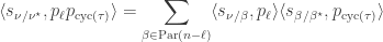
Proposition 5.1 in this joint paper with Anton Evseev and Rowena Paget, restated in the language of symmetric functions is the following recurrence for the plethysm multiplicities relevant to Foulkes’ Conjecture:

Our proof of Proposition 5.1 uses the theory of character deflations, as developed earlier in the paper, together with Frobenius reciprocity.
Generalizations of the Foulkes recurrence
My former Ph.D. student Jasdeep Kochhar used character deflations to prove a considerable generalization, in which  is replaced with an arbitrary partition, and
  with an arbitrary hook partition. I think the only reason he stopped at hook partitions was that this was the only case where there was a convenient combinatorial interpretation of a certain inner product (see the end of this subsection), because his argument easily generalizes to show that
where  is any partition of , the first sum is over all
  (as before) and the second sum is over all
  . Since a one part partition has a unique -hook, if
  then the only relevant
  is
is  . Hence a special case of Kochhar’s result, that generalizes the original result in only one direction, is

with the same condition on the sum over  . In the special case where
  , the plethystic Murnaghan–Nakayama rule states that

and substituting appropriately we recover the original result. More generally, Theorem 6.3 in the joint paper implies that if is a hook partition then  is the product of
  and the size of a certain set of
  border-strip tableaux in which all the border strips have length .
Kochhar’s recurrence can be generalized still further, replacing  and with skew partitions
  and
and  . Below we will prove
  :
:

where  is a skew partition of
  , and the sums are over all and such that ,
  and
and  are skew partitions.
Preliminaries for a symmetric functions proof of ( )
)
We will use several times that if  and
and  are symmetric functions of degrees
  and
and  , and is a partition of
  then
then

One nice proof uses that the coproduct  on the ring of symmetric functions satisfies
  and the general fact
expressing that the coproduct is the dual of multiplication — here one must think of multiplication as the linear map defined by  .
.
Let  be the power sum symmetric function labelled by the partition
  . The expansion of an arbitrary homogeneous symmetric function of degree in the power sum basis is given by

where  is the size of the centralizer of an element
  of cycle type in the symmetric group
  . (This is in fact the most useful definition for our purposes, but there is also the explicit formula
  , where
  is the number of parts of size
  in , or equivalently, the number of -cycles in .) The symmetric functions version of the Murnaghan–Nakayama rule is
where  is the symmetric group character canonically labelled by the skew partition . Thus

expresses a general Schur function in the power sum basis. More typically the Murnaghan–Nakayama rule is applied inductively by repeatedly removing hooks: if  then, the coproduct relation implies that
and hence interpreting each side as a character value, we get the familiar relation

where  is an -cycle disjoint from
  .
.
A symmetric functions proof of ()
Expressing  in the power sum basis we get
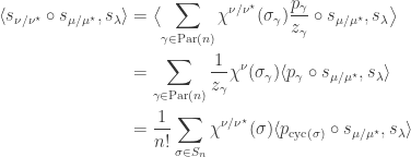
To continue we proceed as in both Kochhar’s proof and the proof of the original Foulkesian recurrence by splitting up the sum according to the length of the cycle of  containing . There are
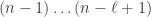
ways to choose elements  to define an -cycle containing ; we must then choose a permutation of the remaining
  elements. We saw in the preliminaries that, by the Murnaghan–Nakayama rule, if is an -cycle then
  . Hence the right-hand side displayed above is

We now use that  for any symmetric functions
  (this is clear for with positive integer monomial coefficients from the interpretation of plethysm as ‘substitute monomials for variables’) and an application the coproduct relation from the preliminaries to get

Repeating the first steps in the proof in reverse order in the inductive case for , this becomes

where the sums are as before. This completes the proof.
Stability of Foulkes Coefficients
I’m in the process of typing up a joint paper with my collaborator Rowena Paget where we prove a number of stability results on plethysm coefficients. Here I’ll show the method using the plethysm  relevant to Foulkes’ Conjecture.
Let  be the set of semistandard tableaux of shape . This set is totally ordered by setting
  if and only if, in the rightmost column in which
  and
and  differ, the larger entry occurs in rather than . Identifying semistandard tableaux of shape
  with -subsets of
  , this order becomes the colexicographic order on sets; similarly identifying semistandard tableaux of shape with -multisubsets of , it becomes the colexicographic order on multisets. An initial segment of
  when
when  is shown below.

Plethystic semistandard tableaux
We can now give the key definition.
Definition. Let be a partition of and let be a partition of . A plethystic semistandard tableaux of shape  is a -tableau with entries from the set , such that the -tableau entries are weakly increasing order along the rows, and strictly increasing order down the columns, with respect to the total order .
Definition. The weight of a plethystic semistandard tableau is the sum of the weights of its -tableau entries.
Let  denote the set of plethystic semistandard tableaux of shape and weight
  . For example the three elements of
  are shown below.

It is a nice exercise to show that the set  is in bijection with the set of partitions of
  contained in an
  box, by the map sending a partition of to the plethystic semistandard tableau whose th largest -tableau entry has exactly
  entries equal to
  (the rest must then be ).
Monomial coefficients in plethysms
The Schur function  enumerates semistandard -tableaux by their weight. Working with variables
  and writing, as is common,
  for
for  , we have
In close analogy, the plethsym  enumerates plethystic semistandard tableau of shape by their weight. With the analogous definition of
  for a plethystic semistandard tableau, we have

Let  denote the monomial symmetric function labelled by the partition . (We avoid the usual notation
  since is in use as the size of .) For instance
It is immediate from the previous displayed equation that the coefficient of the monomial symmetric function in is  . Moreover, by the duality
![\displaystyle \langle \mathrm{mon}_\lambda, h_\alpha \rangle = [\lambda = \alpha]](https://s0.wp.com/latex.php?latex=%5Cdisplaystyle+%5Clangle+%5Cmathrm%7Bmon%7D_%5Clambda%2C+h_%5Calpha+%5Crangle+%3D+%5B%5Clambda+%3D+%5Calpha%5D&bg=ffffff&fg=333333&s=0&c=20201002)
(stated using an Iverson bracket) between the monomial symmetric functions and the complete homogeneous symmetric functions  , we have

This equation  is the critical bridge we need from the combinatorics of plethystic semistandard tableaux to the decomposition of the plethysm into Schur functions.
Two row constituents in the Foulkes plethysm
As an immediate example, we use the suggested exercise above to find the multiplicities  . We require the following lemma.
Lemma. If  then
then  .
.
Stated as above, perhaps the quickest proof of the lemma is to apply the Jacobi—Trudi formula. Recast as a result about characters of the symmetric group, the lemma says that  , where
  is the permutation character of
  acting on -subsets of
  . This leads to an alternative proof by orbit counting.
Proposition. We have  , where
  is the number of partitions of contained in an box.
Proof. This is immediate from the lemma above and equation . 
In particular, it follows by conjugating partitions that if  then the multiplicities of
  in
in  and
and  agree: this verifies Foulkes’ Conjecture in the very special case of two row partitions. Moreover, specializing to two variables, it follows by conjugating partitions that

This is a combinatorial statement of Hermite reciprocity. More explicitly, since  is contained in
  which, by Young’s rule, has only constituents with at most parts, we have

where the sum ends with  if is even, or
  if is odd.
Stable constituents in the Foulkes plethysm
By the proposition above, if  and
and  , then the multiplicity of
  in , is equal to
  , independently of and . The following theorem generalizes this stability result to arbitrary partitions. It was proved, using the partition algebra, as Theorem A in The partition algebra and plethysm coefficients by Chris Bowman and Rowena Paget. I give a very brief outline of their proof in the third section below.
Given a partition of , and  , let
, let ![\gamma_{[d]}](https://s0.wp.com/latex.php?latex=%5Cgamma_%7B%5Bd%5D%7D&bg=ffffff&fg=333333&s=0&c=20201002) denote the partition
denote the partition  . To avoid an unnecessary restriction in the theorem below we also define
 ![(1)_{[1]} = (1)](https://s0.wp.com/latex.php?latex=%281%29_%7B%5B1%5D%7D+%3D+%281%29&bg=ffffff&fg=333333&s=0&c=20201002) . For example, the lemma in the previous section that can now be stated more cleanly as
. For example, the lemma in the previous section that can now be stated more cleanly as ![s_{(r)_{[mn]}} = h_{(r)_{[mn]}} - h_{(r-1)_{[mn]}}](https://s0.wp.com/latex.php?latex=s_%7B%28r%29_%7B%5Bmn%5D%7D%7D+%3D+h_%7B%28r%29_%7B%5Bmn%5D%7D%7D+-+h_%7B%28r-1%29_%7B%5Bmn%5D%7D%7D&bg=ffffff&fg=333333&s=0&c=20201002) . We generalize this in the first lemma following the theorem below.
. We generalize this in the first lemma following the theorem below.
Theorem [Foulkes stability] Let be a partition of . The multiplicity ![\langle s_n \circ s_m, s_{\gamma_{[mn]}} \rangle](https://s0.wp.com/latex.php?latex=%5Clangle+s_n+%5Ccirc+s_m%2C+s_%7B%5Cgamma_%7B%5Bmn%5D%7D%7D+%5Crangle&bg=ffffff&fg=333333&s=0&c=20201002) is independent of and for
is independent of and for  .
.
To prove the Foulkes stability theorem we need two lemmas. I am grateful to Martin Forsberg Conde for pointing out that the stability property in the first lemma is critical to the proof and should be emphasised.
Lemma [Schur/homogeneous stability]. Fix  and
and  . Let
. Let  . For each partition
  there exist unique coefficients
  for
for  such that
![s_{\gamma_{[d]}} = \sum_{\beta \in L} b_{\beta} h_{\beta_{[d]}}.](https://s0.wp.com/latex.php?latex=s_%7B%5Cgamma_%7B%5Bd%5D%7D%7D+%3D+%5Csum_%7B%5Cbeta+%5Cin+L%7D+b_%7B%5Cbeta%7D+h_%7B%5Cbeta_%7B%5Bd%5D%7D%7D.&bg=ffffff&fg=333333&s=0&c=20201002)
Moreover  and
and  unless
  .
.
Proof. Going in the opposite direction, we have
![h_{\beta_{[d]}} = \sum_{\gamma \in L} K_{\beta_{[d]}\gamma_{[d]}} s_{\gamma_{[d]}}, (\ddagger)](https://s0.wp.com/latex.php?latex=h_%7B%5Cbeta_%7B%5Bd%5D%7D%7D+%3D+%5Csum_%7B%5Cgamma+%5Cin+L%7D+K_%7B%5Cbeta_%7B%5Bd%5D%7D%5Cgamma_%7B%5Bd%5D%7D%7D+s_%7B%5Cgamma_%7B%5Bd%5D%7D%7D%2C+%28%5Cddagger%29&bg=ffffff&fg=333333&s=0&c=20201002)
where the Kostka number  is the number of semistandard Young tableaux of shape and content . Since
  unless
  , we are justified in summing only over elements of
  in
in  .
.
Let  be the set of semistandard tableaux of shape
 ![\beta_{[d]}](https://s0.wp.com/latex.php?latex=%5Cbeta_%7B%5Bd%5D%7D&bg=ffffff&fg=333333&s=0&c=20201002) and content . Let . Observe that in any
and content . Let . Observe that in any  , there are
  entries of , and since
  , these s fill up the first row of beyond the end of the second part
  . This leaves
  boxes in the top row to be occupied by entries
  , where the only restriction is that these entries are weakly increasing. Therefore there is a bijection between and the set of semistandard tableaux of disjoint skew-shape
  and content . It follows that
![K_{\beta_{[d]}\gamma_{[d]}} = \widetilde{K}_{\beta\gamma},](https://s0.wp.com/latex.php?latex=K_%7B%5Cbeta_%7B%5Bd%5D%7D%5Cgamma_%7B%5Bd%5D%7D%7D+%3D+%5Cwidetilde%7BK%7D_%7B%5Cbeta%5Cgamma%7D%2C&bg=ffffff&fg=333333&s=0&c=20201002)
independently of  . Moreover, since
  , we have
  , and since unless , we have
  unless
  . The lemma now follows by inverting the unitriangular matrix
  .
.
Lemma [PSSYT stability]. Fix . For each partition with  , the size of the set
 ![\mathrm{PSSYT}\bigl((n), (m)\bigr)_{\gamma_{[mn]}}](https://s0.wp.com/latex.php?latex=%5Cmathrm%7BPSSYT%7D%5Cbigl%28%28n%29%2C+%28m%29%5Cbigr%29_%7B%5Cgamma_%7B%5Bmn%5D%7D%7D&bg=ffffff&fg=333333&s=0&c=20201002) is independent of and , provided that and .
is independent of and , provided that and .
Outline proof. Observe that if  then any -tableau entry in a plethystic semistandard tableau of shape
  and weight
 ![\gamma_{[mn]}](https://s0.wp.com/latex.php?latex=%5Cgamma_%7B%5Bmn%5D%7D&bg=ffffff&fg=333333&s=0&c=20201002) has as its leftmost entry. Similarly, if
has as its leftmost entry. Similarly, if  then the first -tableau entry in such a plethystic semistandard tableau is the all-ones tableau. This shows how to define a bijection between the sets
 ![\mathrm{PSSYT}\bigl((n),(m))_{\gamma_{[mn]}}](https://s0.wp.com/latex.php?latex=%5Cmathrm%7BPSSYT%7D%5Cbigl%28%28n%29%2C%28m%29%29_%7B%5Cgamma_%7B%5Bmn%5D%7D%7D&bg=ffffff&fg=333333&s=0&c=20201002) and
and ![\mathrm{PSSYT}\bigl((n-1),(m-1)\bigr)_{\gamma_{[(m-1)(n-1)]}}](https://s0.wp.com/latex.php?latex=%5Cmathrm%7BPSSYT%7D%5Cbigl%28%28n-1%29%2C%28m-1%29%5Cbigr%29_%7B%5Cgamma_%7B%5B%28m-1%29%28n-1%29%5D%7D%7D&bg=ffffff&fg=333333&s=0&c=20201002) .
.
We are now ready to prove the Foulkes stability theorem.
Proof of Foulkes stability theorem Let . By the lemma on homogeneous/Schur stability, it is sufficient to prove that for each partition such that  or
or  , the multiplicities
 ![\langle s_n \circ s_m, h_{\beta_{[mn]}}\rangle](https://s0.wp.com/latex.php?latex=%5Clangle+s_n+%5Ccirc+s_m%2C+h_%7B%5Cbeta_%7B%5Bmn%5D%7D%7D%5Crangle&bg=ffffff&fg=333333&s=0&c=20201002) are independent of and . This is immediate from equation and the second lemma on PSSYT stability.
are independent of and . This is immediate from equation and the second lemma on PSSYT stability.
Stability for more general plethysms
Let  be the set of integer sequences
  such that
  for all
  and
and  . Given
  and a partition such that
  is also a partition, we define
  to be the maximum number of single box moves, always from longer rows to shorter rows, that take the Young diagram of to the Young diagram of
  .
.
For instance when  and
and  , the maximum number of moves is
  : the unique longer sequence moves one box from row to row , then three boxes from row to row
  , then one box from row to row
  , and finally one box from row
  to row . The sequence of partitions is
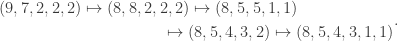
We leave it to the reader to check that  ; since one box must be moved directly from row to row , the move sequence above is no longer feasible.
As background and motivation, we remark that is the weight space of the Lie algebra  , and an upper bound for is the minimal length
  of an expression for
  as a sum of the basic roots
  . For instance, again with we have

corresponding to the move sequence above, and  . In general, we have
  , or, equivalently,
Remark. Brion uses this Lie theoretic interpretation the stability part of the claim below as Theorem 3.1(ii) in his paper Stable properties of plethysm. Part (i) proves that the multiplicity is increasing, while (iii) gives a geometric interpretation of the stable multiplicity.
Claim Let be a partition and let  be such that is also a partition. Let
  . The plethysm coefficient
  is constant for
  and the stable value is
  .
.
Our proof again uses the machine of plethystic semistandard tableaux and stable weight space multiplicities, as computed by taking the inner product with complete homogeneous symmetric functions. As a final remark, note that if  for a partition then
  and the claim gives the stability bound in the Foulkes case originally due to Bowman and Paget and proved above.
The partition algebra and stability
Let  be the natural representation of the general linear group
  . In conventional Schur—Weyl duality, one uses the bimodule
  , acted on diagonally by on the left and by place permutation by
  on the right to pass between polynomial representations of of degree and representations of . The key property that makes this work is that the two actions commute, and, stronger, they have the double centralizer property:

It follows that when one restricts the left action of by replacing the general linear group with a smaller subgroup, the group algebra  must be replaced with some larger algebra. For the orthogonal group one obtains the Brauer algebra, and restricting all the way to the symmetric group
  , one obtains the partition algebra (each defined with parameter ). In the recent meeting at Oberwolfach, Mike Zabrocki commented that he expected new progress on plethysm problems to be made by applying Schur—Weyl-duality in these variants. Incidentally, I highly recommend Zabrocki’s Introduction to symmetric functions for an elegant modern development of the subject.
An outline of the Bowman—Paget method
Given a partition of , let  be the collection of set partitions of
  into disjoint sets of sizes
  . The symmetric group acts transitively on each ; let
  be the corresponding permutation module defined over
  and let
  be the corresponding permutation character. For instance the permutation character appearing in Foulkes’ Conjecture of acting on set partitions of into sets each of size is
  . In this case, each set partition in
  has stabiliser
  ; in general a stabiliser is a direct product of wreath products acting on disjoint subsets.
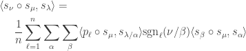
Let  denote the set of partitions of into parts all of size at least . The following theorem is an equivalent restatement of Theorem 8.9 in the paper of Bowman and Paget cited above.
Theorem [Bowman—Paget 2018]. Let be a partition of and let . The stable multiplicity ![\langle s_{(n)} \circ s_{(m)}, s_{\gamma_{[mn]}}\rangle](https://s0.wp.com/latex.php?latex=%5Clangle+s_%7B%28n%29%7D+%5Ccirc+s_%7B%28m%29%7D%2C+s_%7B%5Cgamma_%7B%5Bmn%5D%7D%7D%5Crangle&bg=ffffff&fg=333333&s=0&c=20201002) is equal to
is equal to  .
.
The proof is an impressive application of Schur—Weyl duality and the partition algebra. In outline, the authors start by interpreting the left-hand side as the multiplicity of the Specht module ![S^{\gamma_{[mn]}}](https://s0.wp.com/latex.php?latex=S%5E%7B%5Cgamma_%7B%5Bmn%5D%7D%7D&bg=ffffff&fg=333333&s=0&c=20201002) in the permutation module
in the permutation module  . They then apply Schur—Weyl duality to move to the partition algebra, defined with parameter
  . In this setting, the Specht module becomes the standard module
  for the partition algebra canonically labelled by . Conveniently this module is simply the inflation of the Specht module
  from to the partition algebra. By constructing a filtration of the partition algebra module
  corresponding to , they are able to show that
![[V^{(m^n)} : \Delta_r(\gamma)]_{S_{mn}} = \sum_{\beta \in \mathrm{Par}_{\ge 2}(r)} [P^\beta : S^\gamma]_{S_r}.](https://s0.wp.com/latex.php?latex=%5BV%5E%7B%28m%5En%29%7D+%3A+%5CDelta_r%28%5Cgamma%29%5D_%7BS_%7Bmn%7D%7D+%3D+%5Csum_%7B%5Cbeta+%5Cin+%5Cmathrm%7BPar%7D_%7B%5Cge+2%7D%28r%29%7D+%5BP%5E%5Cbeta+%3A+S%5E%5Cgamma%5D_%7BS_r%7D.&bg=ffffff&fg=333333&s=0&c=20201002)
Restated using characters, this is the version of their theorem stated above. Bowman and Paget also show that depends on the parameters and only through their product (provided, as ever, ); this gives an exceptionally elegant proof that the stable multiplicities for and  agree.
A new result obtained by the partition algebra
Using the method of Bowman and Paget I can prove the analogous results for the stable multiplicities in the plethysm  . Here it is very helpful that the natural representation of decomposes as
  , making it not too hard to describe all the embeddings of the representation
  into the tensor product .
For the  case, the analogue of the set is the set
  of set partitions of
  into disjoint sets of sizes
  , now with one subset marked. Let
  be the corresponding permutation character. Let
  be the set of partitions of with one marked part, and at most one part of size ; if there is a part of size , it must be the unique marked part, and only the first part of a given size may be marked.
Theorem. Let be a partition of and let  . The multiplicity
 ![\langle s_{(n-1,1)} \circ s_{(m)}, s_{\gamma_{[mn]}}\rangle](https://s0.wp.com/latex.php?latex=%5Clangle+s_%7B%28n-1%2C1%29%7D+%5Ccirc+s_%7B%28m%29%7D%2C+s_%7B%5Cgamma_%7B%5Bmn%5D%7D%7D%5Crangle&bg=ffffff&fg=333333&s=0&c=20201002) is stable for
is stable for  and . The stable multiplicity is equal to
  .
.
As a quick example, the marked partitions  lying in
  are
are  ,
,  and
and  with corresponding permutation modules induced from
  ,
,  , and
, and  . (This example is atypical in that the subgroups are all Young subgroups; in general they are products of wreath products.) The sum of the permutation charaters is
  from which one can read off the stable multiplicities of
 ![s_{\gamma_{[mn]}}](https://s0.wp.com/latex.php?latex=s_%7B%5Cgamma_%7B%5Bmn%5D%7D%7D&bg=ffffff&fg=333333&s=0&c=20201002) in . For instance
in . For instance ![s_{(4)_{[mn]}}](https://s0.wp.com/latex.php?latex=s_%7B%284%29_%7B%5Bmn%5D%7D%7D&bg=ffffff&fg=333333&s=0&c=20201002) has stable multiplicity .
has stable multiplicity .
A generalization
This result can be generalized replacing with an arbitrary partition. It turned out that Bowman and Paget had already proved this generalization (with possibly stronger than required bounds on and ) and had a still more general result in which could also be varied, a problem I had no idea how to attack. I’m very happy that we agreed to combine our methods in this joint paper.
Here I’ll record some parts of my original approach. Let  be the set of pairs
  where is a partition of some
  having exactly parts and is a partition of
  into parts all of size . We say that the elements of are -marked partitions. Each -marked partition is determined by the pair of tuples
  and
and  , where is the multiplicity of as a part of and
  is the multiplicity of
  as a part of .
Observe that  is a Young subgroup of
  and
and  is a subgroup of
  , where
  , and
, and  has its conventional meaning.
Given a partition of having exactly parts, we define a map from the characters of to the characters of by a composition of restriction, then inflation then induction. Starting with a character  of , restrict to the Young subgroup
  . Then inflate to the product of wreath products . Finally induce the inflated character up to . We denote the composite map by

Theorem. Let  be a partition of with first part and let be a partition of . Let . The multiplicity
 ![\langle s_{\kappa_{[n]}} \circ s_{(m)}, s_{\gamma_{[mn]}}\rangle](https://s0.wp.com/latex.php?latex=%5Clangle+s_%7B%5Ckappa_%7B%5Bn%5D%7D%7D+%5Ccirc+s_%7B%28m%29%7D%2C+s_%7B%5Cgamma_%7B%5Bmn%5D%7D%7D%5Crangle&bg=ffffff&fg=333333&s=0&c=20201002) is stable for
is stable for  and . The stable multiplicity is equal to

where the character  is defined by
 .
.
We remark that the -marked partition of are in obvious bijection with the partitions of having no singleton parts, and in this case the character  in the left-hand side of the inner product in the theorem is
This is the permutation character of acting on set partitions of into disjoint sets of sizes  . Therefore the case
  of the theorem recovers the original result of Bowman and Paget.
Similarly, a -marked partition  has
has  for a unique ; this defines a unique marked part of size in a corresponding marked partition
  in the sense of the previous section. In this case

which is the permutation character  from the previous section. Therefore again the theorem specializes as expected.
Extended example
We find all stable constituents of the plethysm  when
when  . It will be convenient shorthand to write
  for the Young permutation character induced from the trivial representation of the Young subgroup
  . The decomposition of each is given by the Kostka numbers seen earlier in this post.
The set  has five marked set partitions.
(1)  : here

and

(2)  : here
  and so we compute

The summands inflate to  and
and  , respectively. More simply, these are
  and
and  . Hence

Observe that the right-hand side is  . (This is a bit of a coincidence I think, but convenient for calculation.) Therefore
  and
and
(3)  . A similar argument to the previous case shows that

and since this character is  ,
,

(4)  : here
  and so we compute
  . Inflating and inducing we find that

and since this character is  , we have

(5)  : here
  and so the restriction map does nothing. We then inflate to get
  . The induction of this character to
  is
is

(These constituents can be computed using symmetric functions to evaluate the plethysm  .) The displayed character above is
  .
.
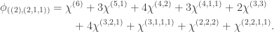
We conclude that, provided  and
and  ,
,
![\begin{aligned} & s_{(n-3,2,1)} \circ s_{(m)} = \\ &\quad \cdots + 4s_{(6)_{[mn]}} \!+\! 11s_{(5,1)_{[mn]}} \!+\! 11s_{(4,2)_{[mn]}} \!+\! 7s_{(4,1,1)_{[mn]}} \\ &\qquad \!+\! 4s_{(3,3)_{[mn]}} \!+\! 8s_{(3,2,1)_{[mn]}} \!+\! s_{(3,1,1,1)_{[mn]}} \!+\! s_{(2,2,2)_{[mn]}}\\ &\qquad \!+\! s_{(2,2,1,1)_{[mn]}} \!+\! \cdots \end{aligned}](https://s0.wp.com/latex.php?latex=%5Cbegin%7Baligned%7D+%26+s_%7B%28n-3%2C2%2C1%29%7D+%5Ccirc+s_%7B%28m%29%7D+%3D+%5C%5C+%26%5Cquad+%5Ccdots+%2B+4s_%7B%286%29_%7B%5Bmn%5D%7D%7D+%5C%21%2B%5C%21+11s_%7B%285%2C1%29_%7B%5Bmn%5D%7D%7D+%5C%21%2B%5C%21+11s_%7B%284%2C2%29_%7B%5Bmn%5D%7D%7D+%5C%21%2B%5C%21+7s_%7B%284%2C1%2C1%29_%7B%5Bmn%5D%7D%7D+%5C%5C+%26%5Cqquad+%5C%21%2B%5C%21+4s_%7B%283%2C3%29_%7B%5Bmn%5D%7D%7D++%5C%21%2B%5C%21+8s_%7B%283%2C2%2C1%29_%7B%5Bmn%5D%7D%7D+%5C%21%2B%5C%21+s_%7B%283%2C1%2C1%2C1%29_%7B%5Bmn%5D%7D%7D+%5C%21%2B%5C%21+s_%7B%282%2C2%2C2%29_%7B%5Bmn%5D%7D%7D%5C%5C+%26%5Cqquad++%5C%21%2B%5C%21+s_%7B%282%2C2%2C1%2C1%29_%7B%5Bmn%5D%7D%7D+%5C%21%2B%5C%21+%5Ccdots+%5Cend%7Baligned%7D&bg=ffffff&fg=333333&s=0&c=20201002)
where the omitted terms are for partitions  where
where  . This decomposition can be verified in about 30 seconds using Magma.
Some corollaries
Setting  we have
![\langle s_{\kappa_{[n]}} \circ s_{(m)}, s_{\gamma_{[mn]}} \rangle = \langle \psi^\kappa_r, \chi^\gamma \rangle.](https://s0.wp.com/latex.php?latex=%5Clangle+s_%7B%5Ckappa_%7B%5Bn%5D%7D%7D+%5Ccirc+s_%7B%28m%29%7D%2C+s_%7B%5Cgamma_%7B%5Bmn%5D%7D%7D+%5Crangle+%3D+%5Clangle+%5Cpsi%5E%5Ckappa_r%2C+%5Cchi%5E%5Cgamma+%5Crangle.&bg=ffffff&fg=333333&s=0&c=20201002)
Plethysms when has two rows. When  we have, for each partition of ,

This is the permutation character of acting on set partitions of  into parts of sizes ,
  ,
,  . Hence
is the permutation character of acting on set partitions of into (non-singleton) parts of sizes and further distinguished parts of sizes  . Denote this character by
  . By the restated version of the theorem,
![\langle s_{(k)_{[n]}} \circ s_{(m)}, s_\gamma \rangle = \sum_{(\alpha,\beta)\in\mathrm{MPar}_k(r)} \langle \rho^{(\alpha,\beta)}, \chi^\gamma\rangle.](https://s0.wp.com/latex.php?latex=%5Clangle+s_%7B%28k%29_%7B%5Bn%5D%7D%7D+%5Ccirc+s_%7B%28m%29%7D%2C+s_%5Cgamma+%5Crangle+%3D+%5Csum_%7B%28%5Calpha%2C%5Cbeta%29%5Cin%5Cmathrm%7BMPar%7D_k%28r%29%7D+%5Clangle+%5Crho%5E%7B%28%5Calpha%2C%5Cbeta%29%7D%2C+%5Cchi%5E%5Cgamma%5Crangle.&bg=ffffff&fg=333333&s=0&c=20201002)
In particular, taking  we find that
![\langle s_{(k)_{[n]}} \circ s_{(m)}, 1_{S_r}\rangle = |\mathrm{MPar}_k(r)|,](https://s0.wp.com/latex.php?latex=%5Clangle+s_%7B%28k%29_%7B%5Bn%5D%7D%7D+%5Ccirc+s_%7B%28m%29%7D%2C+1_%7BS_r%7D%5Crangle+%3D+%7C%5Cmathrm%7BMPar%7D_k%28r%29%7C%2C&bg=ffffff&fg=333333&s=0&c=20201002)
provided that  and . This result may also be proved using plethystic semistandard tableaux: the left-hand side of the previous displayed equation is
  which we have seen is

There is a bijection between plethystic semistandard tableaux  and partitions of into marked parts and some further unmarked parts: the marked parts record the number of s in each -tableau in the second row of . The subtraction in the displayed equation above cancels those partitions having an unmarked singleton part, and so we are left with
  , as required.
Stable hook constituents of  . It is known that a plethysm has a hook constituent if and only if both and are hooks. A particularly beautiful proof of this result, using the plethystic substitution
 ![s_\nu[1-X]](https://s0.wp.com/latex.php?latex=s_%5Cnu%5B1-X%5D&bg=ffffff&fg=333333&s=0&c=20201002) , was given by Langley and Remmel: see Theorem 3.1 in their paper The plethysm
, was given by Langley and Remmel: see Theorem 3.1 in their paper The plethysm ![s_\lambda[s_\mu]](https://s0.wp.com/latex.php?latex=s_%5Clambda%5Bs_%5Cmu%5D&bg=ffffff&fg=333333&s=0&c=20201002) at hook and near-hook shapes. In particular, the only hook that appears in the Foulkes plethysm is
at hook and near-hook shapes. In particular, the only hook that appears in the Foulkes plethysm is  .
.
Here we consider the analogous result for stable hooks, i.e. partitions of the form  . To get started take . Let
  . Since
  is a Littlewood–Richardson product of the transitive permutation characters
  for
for  , and a Littlewood–Richardson product is a hook only when every term in the product is a hook, the stable hook constituents
  are precisely the hook partitions in

Therefore  is the number of semistandard Young tableaux of shape and content
  . This is the Kostka number
In particular, the longest leg length occurs when the content is  , and so the longest leg length of a stable hook grows as
  . (We emphasise that all this follows from the original result of Bowman and Paget.)
If we replace with  , using the generalization proved above, then the marked parts in a marked partition
  contributes further parts
  to the content above, and so the stable hook multiplicity is

For example taking , the stable  -hooks in are
  with multiplicity , and
  with multiplicity . The elements of
  are
are  ,
,  ,
,  ,
,  , of which the final three each defines a unique semistandard Young tableau counted by the Kostka number above; the contents are
  ,
,  and
and  respectively.


 Posted by mwildon
  . We define the
  to be the number of
  . If
. If  or
or  then, by definition, the
  for a varying
  .
. be a given
  . The number of
  .
. be the canonical basis of
  has a unique basis (up to order) of the form
 . There are
  choices for each of
  and so
  followed by a basis for
  we obtain a matrix
 correspond to distinct subspaces
  is
is  .
. is an
is an  -dimensional subspace of
  containing
  . Hence there are
  -choices for a subspace
  in which
  .
. be given
  . The number of
  is
is  .
. , there are
  complementary subspaces
  to
to  . Now again use that subspaces of the quotient space
  are in bijection with subspaces of
 -dimensional subspace
  of
of  having intersection of dimension
  with
with  and
and  , there are
  such subspaces. Summing over
  , else
 and
and  in the original version, cancel in a few places, swap the order of the binomial coefficients in each product, and then erase the primes.
  induced by applying the unit on
  to get a canonical inclusion
  .
. and let Vect be the category of
  defined by
  maps to ‘evaluate at
 ![v \stackrel{\eta_V}{\longmapsto} [\theta \mapsto \theta(v)]\qquad(\star)](https://s0.wp.com/latex.php?latex=v+%5Cstackrel%7B%5Ceta_V%7D%7B%5Clongmapsto%7D+%5B%5Ctheta+%5Cmapsto+%5Ctheta%28v%29%5D%5Cqquad%28%5Cstar%29&bg=ffffff&fg=333333&s=0&c=20201002)
 and
and  . Thus
  from the identity functor on Vect to the double dual functor
  is a vastly bigger vector space than
  is the vector space of all
  . Moreover
  . (Even the existence of bases for
  it is implied by the Boolean Prime Ideal Theorem, a weak form of the Axiom of Choice.) For this reason we have to reason formally, mainly by manipulating symbols, rather than use matrices or bases. But this is a good thing: for instance it means our formulae for the monad unit and monad multiplication translates entirely routinely to define the continuation monad in the category Hask.
 . Thus for each vector space
  . As already said, we obtain this as the dual map to
  . That is
 is the linear map
 ![\theta \stackrel{\eta_{V^\star}}{\longmapsto} [\phi \mapsto \phi(\theta)]](https://s0.wp.com/latex.php?latex=%5Ctheta+%5Cstackrel%7B%5Ceta_%7BV%5E%5Cstar%7D%7D%7B%5Clongmapsto%7D+%5B%5Cphi+%5Cmapsto+%5Cphi%28%5Ctheta%29%5D&bg=ffffff&fg=333333&s=0&c=20201002)
 and
and  . Generally, given a linear map
  , the dual map is given by `restriction along
  as an element of
  by mapping
  into
into  by
by  ; in symbols
  . Therefore the dual map to
 ![w \stackrel{\mu_V}{\longmapsto} [\theta \mapsto w(\eta_{V^\star}(\theta))] = [\theta \mapsto w([\phi \mapsto \phi(\theta)])] \quad (\dagger)](https://s0.wp.com/latex.php?latex=w+%5Cstackrel%7B%5Cmu_V%7D%7B%5Clongmapsto%7D+%5B%5Ctheta+%5Cmapsto+w%28%5Ceta_%7BV%5E%5Cstar%7D%28%5Ctheta%29%29%5D+%3D+%5B%5Ctheta+%5Cmapsto+w%28%5B%5Cphi+%5Cmapsto+%5Cphi%28%5Ctheta%29%5D%29%5D++%5Cquad+%28%5Cdagger%29&bg=ffffff&fg=333333&s=0&c=20201002)

 ; multiplication then becomes the observation that interpreting variables in a boolean formula as yet further boolean formulae does not leave the space of boolean formulae. Here I will note that the definition of
  in
in  is an element of
  and therefore in the domain of
  . Naturality of
 defines a monad. For this we need to check the monad laws shown in the commutative diagrams below.
 . This has a short proof, which, as expected from the remark about formalism above, come down to juggling the order of symbols until everything works out. Recall that
  is the canonical embedding of
  . Thus if we take
  is the element of
  defined by
 . This map sends
 ![[\phi \mapsto \phi(\theta)]](https://s0.wp.com/latex.php?latex=%5B%5Cphi+%5Cmapsto+%5Cphi%28%5Ctheta%29%5D&bg=ffffff&fg=333333&s=0&c=20201002) in
in ![\begin{aligned} (\mu_V \circ \eta_{V^{\star\star}})(\phi) &= \mu_V([\Psi \mapsto \Psi(\phi)]) \\&= [\theta \mapsto (\eta_{V^\star}(\theta))(\phi)] \\ &= [\theta \mapsto \phi(\theta)] \\&= \phi \end{aligned}](https://s0.wp.com/latex.php?latex=%5Cbegin%7Baligned%7D+%28%5Cmu_V+%5Ccirc+%5Ceta_%7BV%5E%7B%5Cstar%5Cstar%7D%7D%29%28%5Cphi%29+%26%3D+%5Cmu_V%28%5B%5CPsi+%5Cmapsto+%5CPsi%28%5Cphi%29%5D%29+%5C%5C%26%3D+%5B%5Ctheta+%5Cmapsto+%28%5Ceta_%7BV%5E%5Cstar%7D%28%5Ctheta%29%29%28%5Cphi%29%5D+%5C%5C+%26%3D+%5B%5Ctheta+%5Cmapsto+%5Cphi%28%5Ctheta%29%5D+%5C%5C%26%3D+%5Cphi+%5Cend%7Baligned%7D&bg=ffffff&fg=333333&s=0&c=20201002)
 is indeed the identity of
  , I will omit it. I plan in a sequel to this post to show that
  is the monad induced by the adjunction betweeen the contravariant dual and itself; the identity monad law then becomes the
  for the right-hand functor
  in the adjunction, and the associativity law becomes an immediate application of the
  is some kind of linear map
  , and since all we have to hand is
  itself? It would be intriguing if this could be made into a rigorous argument either working in Vect or directly in Hask, perhaps using ideas from Wadler’s paper
  , as defined in
  to
to![\mu_V(w) = [\theta \mapsto w(\eta_{V^\star}(\theta))]](https://s0.wp.com/latex.php?latex=%5Cmu_V%28w%29+%3D+%5B%5Ctheta+%5Cmapsto+w%28%5Ceta_%7BV%5E%5Cstar%7D%28%5Ctheta%29%29%5D&bg=ffffff&fg=333333&s=0&c=20201002) to
to  , we have
  or unpacked fully,
 ![f^{\star\star}\phi = [\theta \mapsto \phi(f^\star (\theta))] = \theta \mapsto \phi(\theta \circ f)](https://s0.wp.com/latex.php?latex=f%5E%7B%5Cstar%5Cstar%7D%5Cphi+%3D+%5B%5Ctheta+%5Cmapsto+%5Cphi%28f%5E%5Cstar+%28%5Ctheta%29%29%5D+%3D+%5Ctheta+%5Cmapsto+%5Cphi%28%5Ctheta+%5Ccirc+f%29&bg=ffffff&fg=333333&s=0&c=20201002)
 .
. , but surely the input won’t be, but the true reason is to make a distinction between the types
  maps to evaluate at
  and then
  is evaluated, and so on. (This can be checked using the linked Haskell code, which puts a trace on plus.) Still bad, but more easily fixed, is the left-associative fold
  , and then
  is evaluated, and so on. The correct way to write it uses a strict left-fold, available as
  . Note that although this might look like a left-associative fold, it does the same computation as the right-associative fold.
  by sampling from
 . More precisely, it is
 of the standard normal distribution.
  , we have
 should be well approximated by an exponential distribution with parameter
  , and, correspondingly, as is
  . Thus this approximation suggests that the mean of the tail distribution should be
  and its variance
  or more standard deviations from the mean, in a sample conditioned to be at least
  outliers
 and you have 50 colleagues, then since only 2.3% of the conditioned sample are outliers, lying in the
  tail, there is a good chance that none of your colleagues is more than 1 standard deviation ahead of you in ability.
 we sample from
  we sample from
  (lucky people). Suppose that
  , so the effect of luck is relatively modest, boosting one’s performance by just
  a standard deviation. As before, we then reject all samples below the threshold
  of being lucky. The final column is the ratio of lucky to average people.
 tail of the distribution (with, as just explained, a boost of 0.5 for lucky people), lucky people predominate. The effect is that the University of Erewhon fails in its goal of recruiting people three standard deviations above the mean: instead of the 2230 successful candidate, 1176 are people who are merely about 2.5 standard deviations above the mean, but happened to get lucky.
 random variable, so the standard deviation is
  distribution, the effect is to increase the variance, while leaving the mean unchanged. The graphs below show the probability density function for the original
  tail, for
  .
. 

 (the blue curve) only 10.09% of the conditional probability density function is in the negative half. Almost everyone recruited gets lucky, most by at least one standard deviation from the mean and many by two or more standard deviations from the mean. The moral is again clear: unless you believe (as is sometimes
  and lift the identity
 is the number of
  , working over an arbitrary field
  . We then descend to get quick proofs of generalizations of the symmetric function identity
 and the corresponding
  , namely
![\sum_{r=0}^n (-1)^r q^{r(r-1)2} \genfrac{[}{]}{0pt}{}{n-r+D-1}{n-r}_q \genfrac{[}{]}{0pt}{}{D}{r}_q = 0.](https://s0.wp.com/latex.php?latex=%5Csum_%7Br%3D0%7D%5En+%28-1%29%5Er+q%5E%7Br%28r-1%292%7D+%5Cgenfrac%7B%5B%7D%7B%5D%7D%7B0pt%7D%7B%7D%7Bn-r%2BD-1%7D%7Bn-r%7D_q++%5Cgenfrac%7B%5B%7D%7B%5D%7D%7B0pt%7D%7B%7D%7BD%7D%7Br%7D_q+%3D+0.&bg=ffffff&fg=333333&s=0&c=20201002)
 denote the number of
 . I finish by explaining how my
  over an arbitrary field
  , we define its weight, denoted
  , to be its sum of entries. We shall adopt a slightly unconventional approach and define the
 ![\genfrac{[}{]}{0pt}{}{n}{k}_q \in \mathbb{C}[q]](https://s0.wp.com/latex.php?latex=%5Cgenfrac%7B%5B%7D%7B%5D%7D%7B0pt%7D%7B%7D%7Bn%7D%7Bk%7D_q+%5Cin+%5Cmathbb%7BC%7D%5Bq%5D&bg=ffffff&fg=333333&s=0&c=20201002) to be the enumerator by weight of the
to be the enumerator by weight of the  , normalized to have constant term
 ![\genfrac{[}{]}{0pt}{}{n}{k}_q = q^{-k(k-1)/2} \sum_{X \subseteq \{0,1,\ldots, n-1\}} q^{\mathrm{wt}(X)}.](https://s0.wp.com/latex.php?latex=%5Cgenfrac%7B%5B%7D%7B%5D%7D%7B0pt%7D%7B%7D%7Bn%7D%7Bk%7D_q+%3D+q%5E%7B-k%28k-1%29%2F2%7D+%5Csum_%7BX+%5Csubseteq+%5C%7B0%2C1%2C%5Cldots%2C+n-1%5C%7D%7D+q%5E%7B%5Cmathrm%7Bwt%7D%28X%29%7D.&bg=ffffff&fg=333333&s=0&c=20201002)
![\genfrac{[}{]}{0pt}{}{n}{k}_q = 0](https://s0.wp.com/latex.php?latex=%5Cgenfrac%7B%5B%7D%7B%5D%7D%7B0pt%7D%7B%7D%7Bn%7D%7Bk%7D_q+%3D+0&bg=ffffff&fg=333333&s=0&c=20201002) if
if ![\genfrac{[}{]}{0pt}{}{n}{k}_q](https://s0.wp.com/latex.php?latex=%5Cgenfrac%7B%5B%7D%7B%5D%7D%7B0pt%7D%7B%7D%7Bn%7D%7Bk%7D_q&bg=ffffff&fg=333333&s=0&c=20201002) is a polynomial in
is a polynomial in ![\begin{aligned} \genfrac{[}{]}{0pt}{}{4}{2}_q&= q^{-1}(q^{0+1} + q^{0+2} + q^{0+3} + q^{1+2} + q^{1+3} + q^{2+3}) \\ &= 1 + q + 2q^2 + q^3 + q^4, \end{aligned}](https://s0.wp.com/latex.php?latex=%5Cbegin%7Baligned%7D+%5Cgenfrac%7B%5B%7D%7B%5D%7D%7B0pt%7D%7B%7D%7B4%7D%7B2%7D_q%26%3D+q%5E%7B-1%7D%28q%5E%7B0%2B1%7D+%2B+q%5E%7B0%2B2%7D+%2B+q%5E%7B0%2B3%7D+%2B+q%5E%7B1%2B2%7D+%2B+q%5E%7B1%2B3%7D+%2B+q%5E%7B2%2B3%7D%29+%5C%5C+%26%3D+1+%2B+q+%2B+2q%5E2+%2B+q%5E3+%2B+q%5E4%2C+%5Cend%7Baligned%7D&bg=ffffff&fg=333333&s=0&c=20201002)
![\genfrac{[}{]}{0pt}{}{n}{0}_q = \genfrac{[}{]}{0pt}{}{n}{n}_q = 1](https://s0.wp.com/latex.php?latex=%5Cgenfrac%7B%5B%7D%7B%5D%7D%7B0pt%7D%7B%7D%7Bn%7D%7B0%7D_q+%3D+%5Cgenfrac%7B%5B%7D%7B%5D%7D%7B0pt%7D%7B%7D%7Bn%7D%7Bn%7D_q+%3D+1&bg=ffffff&fg=333333&s=0&c=20201002) and
and ![\genfrac{[}{]}{0pt}{}{n}{1}_q = 1 + q + \cdots + q^{n-1}](https://s0.wp.com/latex.php?latex=%5Cgenfrac%7B%5B%7D%7B%5D%7D%7B0pt%7D%7B%7D%7Bn%7D%7B1%7D_q++%3D+1+%2B+q+%2B+%5Ccdots+%2B+q%5E%7Bn-1%7D&bg=ffffff&fg=333333&s=0&c=20201002) for all
for all  . We now recover the usual definition of
  , which we prove by adapting the standard bijective proof.
 then
then![\genfrac{[}{]}{0pt}{}{n}{k}_q = q^{n-k} \genfrac{[}{]}{0pt}{}{n-1}{k-1}_q + \genfrac{[}{]}{0pt}{}{n-1}{k}_q.](https://s0.wp.com/latex.php?latex=%5Cgenfrac%7B%5B%7D%7B%5D%7D%7B0pt%7D%7B%7D%7Bn%7D%7Bk%7D_q+%3D+q%5E%7Bn-k%7D+%5Cgenfrac%7B%5B%7D%7B%5D%7D%7B0pt%7D%7B%7D%7Bn-1%7D%7Bk-1%7D_q++%2B+%5Cgenfrac%7B%5B%7D%7B%5D%7D%7B0pt%7D%7B%7D%7Bn-1%7D%7Bk%7D_q.&bg=ffffff&fg=333333&s=0&c=20201002)
 then the result holds by our convention that
 ![\genfrac{[}{]}{0pt}{}{n-1}{-1}_q = 0](https://s0.wp.com/latex.php?latex=%5Cgenfrac%7B%5B%7D%7B%5D%7D%7B0pt%7D%7B%7D%7Bn-1%7D%7B-1%7D_q+%3D+0&bg=ffffff&fg=333333&s=0&c=20201002) so we may suppose that
so we may suppose that  . Removing
  from a
  containing
  subsets of
  , enumerated by
 ![\genfrac{[}{]}{0pt}{}{n-1}{k-1}_q](https://s0.wp.com/latex.php?latex=%5Cgenfrac%7B%5B%7D%7B%5D%7D%7B0pt%7D%7B%7D%7Bn-1%7D%7Bk-1%7D_q&bg=ffffff&fg=333333&s=0&c=20201002) . This map decreases the weight by
. This map decreases the weight by ![\genfrac{[}{]}{0pt}{}{n-1}{k}_q](https://s0.wp.com/latex.php?latex=%5Cgenfrac%7B%5B%7D%7B%5D%7D%7B0pt%7D%7B%7D%7Bn-1%7D%7Bk%7D_q&bg=ffffff&fg=333333&s=0&c=20201002) . Therefore,
. Therefore, ![q^{k(k-1)/2} \genfrac{[}{]}{0pt}{}{n}{k}_q = q^{n-1} q^{(k-1)(k-2)/2} \genfrac{[}{]}{0pt}{}{n-1}{k-1}_q + q^{k(k-1)/2} \genfrac{[}{]}{0pt}{}{n-1}{k}_q.](https://s0.wp.com/latex.php?latex=q%5E%7Bk%28k-1%29%2F2%7D+%5Cgenfrac%7B%5B%7D%7B%5D%7D%7B0pt%7D%7B%7D%7Bn%7D%7Bk%7D_q+%3D+q%5E%7Bn-1%7D+q%5E%7B%28k-1%29%28k-2%29%2F2%7D+%5Cgenfrac%7B%5B%7D%7B%5D%7D%7B0pt%7D%7B%7D%7Bn-1%7D%7Bk-1%7D_q+%2B+q%5E%7Bk%28k-1%29%2F2%7D+%5Cgenfrac%7B%5B%7D%7B%5D%7D%7B0pt%7D%7B%7D%7Bn-1%7D%7Bk%7D_q.&bg=ffffff&fg=333333&s=0&c=20201002)
 , using that
![[n]_q](https://s0.wp.com/latex.php?latex=%5Bn%5D_q&bg=ffffff&fg=333333&s=0&c=20201002) by
by ![[n]_q = 1 + q + \cdots + q^{n-1}](https://s0.wp.com/latex.php?latex=%5Bn%5D_q+%3D+1+%2B+q+%2B+%5Ccdots+%2B+q%5E%7Bn-1%7D&bg=ffffff&fg=333333&s=0&c=20201002) and the quantum factorial
and the quantum factorial ![[n]_q!](https://s0.wp.com/latex.php?latex=%5Bn%5D_q%21&bg=ffffff&fg=333333&s=0&c=20201002) by
by ![[n]_q! = [n]_q[n-1]_q \ldots [1]_q](https://s0.wp.com/latex.php?latex=%5Bn%5D_q%21+%3D+%5Bn%5D_q%5Bn-1%5D_q+%5Cldots+%5B1%5D_q&bg=ffffff&fg=333333&s=0&c=20201002) . Observe that specializing
. Observe that specializing  , respectively. (See the section on characters below for the connection with the alternative convention in which quantum numbers are Laurent polynomials.) Note that in the following proposition, if
 ![\genfrac{[}{]}{0pt}{}{n}{0}_q = 1](https://s0.wp.com/latex.php?latex=%5Cgenfrac%7B%5B%7D%7B%5D%7D%7B0pt%7D%7B%7D%7Bn%7D%7B0%7D_q+%3D+1&bg=ffffff&fg=333333&s=0&c=20201002) for all
for all ![\displaystyle\genfrac{[}{]}{0pt}{}{n}{k}_ q = \frac{[n]_q[n-1]_q \ldots [n-k+1]_q}{[k]_q!}.](https://s0.wp.com/latex.php?latex=%5Cdisplaystyle%5Cgenfrac%7B%5B%7D%7B%5D%7D%7B0pt%7D%7B%7D%7Bn%7D%7Bk%7D_+q+%3D+%5Cfrac%7B%5Bn%5D_q%5Bn-1%5D_q+%5Cldots+%5Bn-k%2B1%5D_q%7D%7B%5Bk%5D_q%21%7D.&bg=ffffff&fg=333333&s=0&c=20201002)
 using the previous lemma we have
![\begin{aligned} \genfrac{[}{]}{0pt}{}{n}{k}_q &= q^{n-k}\genfrac{[}{]}{0pt}{}{n-1}{k-1}_q + \genfrac{[}{]}{0pt}{}{n-1}{k}_q \\ &= q^{n-k} \frac{[n-1]_q\ldots [n-k+1]_q[n-k]_q}{[k-1]_q!} \\ &\qquad \qquad \qquad + \frac{[n-1]_q\ldots [n-k+1]_q[n-k]_q}{[k]_q!} \\&= \frac{[n-1]_q\ldots [n-k+1]_q}{[k]_q!} \bigl( q^{n-k}[k]_q + [n-k]_q \bigr) \\ &= \frac{[n-1]_q \ldots [n-k+1]_q}{[k]_q!} [n]_q \\ \end{aligned}](https://s0.wp.com/latex.php?latex=%5Cbegin%7Baligned%7D+%5Cgenfrac%7B%5B%7D%7B%5D%7D%7B0pt%7D%7B%7D%7Bn%7D%7Bk%7D_q+%26%3D++q%5E%7Bn-k%7D%5Cgenfrac%7B%5B%7D%7B%5D%7D%7B0pt%7D%7B%7D%7Bn-1%7D%7Bk-1%7D_q+%2B+%5Cgenfrac%7B%5B%7D%7B%5D%7D%7B0pt%7D%7B%7D%7Bn-1%7D%7Bk%7D_q+%5C%5C+%26%3D+q%5E%7Bn-k%7D+%5Cfrac%7B%5Bn-1%5D_q%5Cldots+%5Bn-k%2B1%5D_q%5Bn-k%5D_q%7D%7B%5Bk-1%5D_q%21%7D+%5C%5C+%26%5Cqquad+%5Cqquad+%5Cqquad+%2B+%5Cfrac%7B%5Bn-1%5D_q%5Cldots+%5Bn-k%2B1%5D_q%5Bn-k%5D_q%7D%7B%5Bk%5D_q%21%7D+%5C%5C%26%3D+%5Cfrac%7B%5Bn-1%5D_q%5Cldots+%5Bn-k%2B1%5D_q%7D%7B%5Bk%5D_q%21%7D+%5Cbigl%28++q%5E%7Bn-k%7D%5Bk%5D_q+%2B+%5Bn-k%5D_q++%5Cbigr%29+%5C%5C+%26%3D+%5Cfrac%7B%5Bn-1%5D_q+%5Cldots+%5Bn-k%2B1%5D_q%7D%7B%5Bk%5D_q%21%7D+%5Bn%5D_q+%5C%5C+%5Cend%7Baligned%7D&bg=ffffff&fg=333333&s=0&c=20201002)
![\begin{aligned} q^{n-k}[k]_q + [n-k]_q &= q^{n-k}(1+q + \cdots + q^{k-1}) \\ & \qquad\qquad + 1 + q + \cdots + q^{n-k-1} \\ &= 1 + q + \cdots + q^{n-1} \\&= [n]_q \end{aligned}](https://s0.wp.com/latex.php?latex=%5Cbegin%7Baligned%7D+q%5E%7Bn-k%7D%5Bk%5D_q+%2B+%5Bn-k%5D_q+%26%3D+q%5E%7Bn-k%7D%281%2Bq+%2B+%5Ccdots+%2B+q%5E%7Bk-1%7D%29++%5C%5C+%26+%5Cqquad%5Cqquad+%2B+1+%2B+q+%2B+%5Ccdots+%2B+q%5E%7Bn-k-1%7D+%5C%5C+%26%3D+1+%2B+q+%2B+%5Ccdots+%2B+q%5E%7Bn-1%7D+%5C%5C%26%3D+%5Bn%5D_q+%5Cend%7Baligned%7D&bg=ffffff&fg=333333&s=0&c=20201002)
![\left[\!\genfrac{[}{]}{0pt}{}{n}{k}\!\right]_q = \sum_M q^{\mathrm{wt}(M)}](https://s0.wp.com/latex.php?latex=%5Cleft%5B%5C%21%5Cgenfrac%7B%5B%7D%7B%5D%7D%7B0pt%7D%7B%7D%7Bn%7D%7Bk%7D%5C%21%5Cright%5D_q+%3D+%5Csum_M+q%5E%7B%5Cmathrm%7Bwt%7D%28M%29%7D&bg=ffffff&fg=333333&s=0&c=20201002)
![\begin{aligned} \left[\!\genfrac{[}{]}{0pt}{}{3}{2}\!\right]_q &= q^{0+0} + q^{0+1} + q^{0+2} + q^{1+1} + q^{1+2} + q^{2+2} \\ &= 1 + q + 2q^2 + q^3 + q^4 \\ &= \genfrac{[}{]}{0pt}{}{4}{2}_q\end{aligned}](https://s0.wp.com/latex.php?latex=%5Cbegin%7Baligned%7D+%5Cleft%5B%5C%21%5Cgenfrac%7B%5B%7D%7B%5D%7D%7B0pt%7D%7B%7D%7B3%7D%7B2%7D%5C%21%5Cright%5D_q++%26%3D+q%5E%7B0%2B0%7D+%2B+q%5E%7B0%2B1%7D+%2B+q%5E%7B0%2B2%7D+%2B+q%5E%7B1%2B1%7D+%2B+q%5E%7B1%2B2%7D+%2B+q%5E%7B2%2B2%7D+%5C%5C+%26%3D+1+%2B+q+%2B+2q%5E2+%2B+q%5E3+%2B+q%5E4++%5C%5C+%26%3D+%5Cgenfrac%7B%5B%7D%7B%5D%7D%7B0pt%7D%7B%7D%7B4%7D%7B2%7D_q%5Cend%7Baligned%7D+&bg=ffffff&fg=333333&s=0&c=20201002)
![\left[\!\genfrac{[}{]}{0pt}{}{n}{0}\!\right]_q = 1](https://s0.wp.com/latex.php?latex=%5Cleft%5B%5C%21%5Cgenfrac%7B%5B%7D%7B%5D%7D%7B0pt%7D%7B%7D%7Bn%7D%7B0%7D%5C%21%5Cright%5D_q+%3D+1&bg=ffffff&fg=333333&s=0&c=20201002) and
and![\left[\!\genfrac{[}{]}{0pt}{}{n}{1}\!\right]_q = q^0 + q^1 + \cdots + q^{n-1} = [n]_q = \genfrac{[}{]}{0pt}{}{n}{1}_q](https://s0.wp.com/latex.php?latex=%5Cleft%5B%5C%21%5Cgenfrac%7B%5B%7D%7B%5D%7D%7B0pt%7D%7B%7D%7Bn%7D%7B1%7D%5C%21%5Cright%5D_q+%3D+q%5E0+%2B+q%5E1+%2B+%5Ccdots+%2B+q%5E%7Bn-1%7D+%3D+%5Bn%5D_q+%3D+%5Cgenfrac%7B%5B%7D%7B%5D%7D%7B0pt%7D%7B%7D%7Bn%7D%7B1%7D_q&bg=ffffff&fg=333333&s=0&c=20201002)
![\left[\!\genfrac{[}{]}{0pt}{}{3}{2}\!\right]_q = \genfrac{[}{]}{0pt}{}{4}{2}_q](https://s0.wp.com/latex.php?latex=%5Cleft%5B%5C%21%5Cgenfrac%7B%5B%7D%7B%5D%7D%7B0pt%7D%7B%7D%7B3%7D%7B2%7D%5C%21%5Cright%5D_q+%3D+%5Cgenfrac%7B%5B%7D%7B%5D%7D%7B0pt%7D%7B%7D%7B4%7D%7B2%7D_q&bg=ffffff&fg=333333&s=0&c=20201002) is not a coincidence.
is not a coincidence. where
where  . In turn, such sequences are in bijection with
  by the map
 to a subset of weight
  . By the first section,
 ![q^{k(k-1)/2}\genfrac{[}{]}{0pt}{}{n+k-1}{k}_q](https://s0.wp.com/latex.php?latex=q%5E%7Bk%28k-1%29%2F2%7D%5Cgenfrac%7B%5B%7D%7B%5D%7D%7B0pt%7D%7B%7D%7Bn%2Bk-1%7D%7Bk%7D_q&bg=ffffff&fg=333333&s=0&c=20201002) enumerates
enumerates ![\left[\!\genfrac{[}{]}{0pt}{}{n}{k}\!\right]_q = \genfrac{[}{]}{0pt}{}{n+k-1}{k}_q .\qquad(2)](https://s0.wp.com/latex.php?latex=%5Cleft%5B%5C%21%5Cgenfrac%7B%5B%7D%7B%5D%7D%7B0pt%7D%7B%7D%7Bn%7D%7Bk%7D%5C%21%5Cright%5D_q+%3D+%5Cgenfrac%7B%5B%7D%7B%5D%7D%7B0pt%7D%7B%7D%7Bn%2Bk-1%7D%7Bk%7D_q+.%5Cqquad%282%29+&bg=ffffff&fg=333333&s=0&c=20201002)
![\left[\!\genfrac{[}{]}{0pt}{}{n}{k}\!\right]_q](https://s0.wp.com/latex.php?latex=%5Cleft%5B%5C%21%5Cgenfrac%7B%5B%7D%7B%5D%7D%7B0pt%7D%7B%7D%7Bn%7D%7Bk%7D%5C%21%5Cright%5D_q&bg=ffffff&fg=333333&s=0&c=20201002) . Observe that a partition whose Young diagram is contained in the
. Observe that a partition whose Young diagram is contained in the  box is uniquely specified by the sequence
  of
of  . Therefore
 corresponds to recording a partition not by the
  and
and  of the partitions
  and
and  are shown in the diagram below with step numbers in bold.
![\genfrac{[}{]}{0pt}{}{n}{k}_q = q^{n-k} \genfrac{[}{]}{0pt}{}{n-1}{k-1}_q + \genfrac{[}{]}{0pt}{}{n-1}{k}_q.](https://s0.wp.com/latex.php?latex=%5Cgenfrac%7B%5B%7D%7B%5D%7D%7B0pt%7D%7B%7D%7Bn%7D%7Bk%7D_q+%3D++q%5E%7Bn-k%7D+%5Cgenfrac%7B%5B%7D%7B%5D%7D%7B0pt%7D%7B%7D%7Bn-1%7D%7Bk-1%7D_q+%2B+%5Cgenfrac%7B%5B%7D%7B%5D%7D%7B0pt%7D%7B%7D%7Bn-1%7D%7Bk%7D_q.&bg=ffffff&fg=333333&s=0&c=20201002)
![\genfrac{[}{]}{0pt}{}{n}{k}_q = \genfrac{[}{]}{0pt}{}{n-1}{k-1}_q + q^k \genfrac{[}{]}{0pt}{}{n-1}{k}_q.](https://s0.wp.com/latex.php?latex=%5Cgenfrac%7B%5B%7D%7B%5D%7D%7B0pt%7D%7B%7D%7Bn%7D%7Bk%7D_q+%3D+%5Cgenfrac%7B%5B%7D%7B%5D%7D%7B0pt%7D%7B%7D%7Bn-1%7D%7Bk-1%7D_q+%2B+q%5Ek+%5Cgenfrac%7B%5B%7D%7B%5D%7D%7B0pt%7D%7B%7D%7Bn-1%7D%7Bk%7D_q.&bg=ffffff&fg=333333&s=0&c=20201002)
![(1 + qz)(1+q^2 z) \ldots (1+q^{n-1}z) = \sum_{k=0}^n q^{k(k-1)/2} \genfrac{[}{]}{0pt}{}{n}{k}_q z^k](https://s0.wp.com/latex.php?latex=%281+%2B+qz%29%281%2Bq%5E2+z%29+%5Cldots+%281%2Bq%5E%7Bn-1%7Dz%29+%3D+%5Csum_%7Bk%3D0%7D%5En+q%5E%7Bk%28k-1%29%2F2%7D+%5Cgenfrac%7B%5B%7D%7B%5D%7D%7B0pt%7D%7B%7D%7Bn%7D%7Bk%7D_q+z%5Ek&bg=ffffff&fg=333333&s=0&c=20201002)
 and
and  be the elementary and complete symmetric functions of degree
  . Thus
 entries of
  then
then  . It is a good basic exercise to show that
  and
and  . It is immediate from our definition of
 ![e_k(1,q,\ldots, q^{n-1}) = q^{k(k-1)/2} \genfrac{[}{]}{0pt}{}{n}{k}_q](https://s0.wp.com/latex.php?latex=e_k%281%2Cq%2C%5Cldots%2C+q%5E%7Bn-1%7D%29+%3D+q%5E%7Bk%28k-1%29%2F2%7D+%5Cgenfrac%7B%5B%7D%7B%5D%7D%7B0pt%7D%7B%7D%7Bn%7D%7Bk%7D_q&bg=ffffff&fg=333333&s=0&c=20201002)
![h_k(1,q,\ldots, q^{n-1}) = \left[\!\genfrac{[}{]}{0pt}{}{n}{k}\!\right] = \genfrac{[}{]}{0pt}{}{n+k-1}{k}_q](https://s0.wp.com/latex.php?latex=h_k%281%2Cq%2C%5Cldots%2C+q%5E%7Bn-1%7D%29+%3D+%5Cleft%5B%5C%21%5Cgenfrac%7B%5B%7D%7B%5D%7D%7B0pt%7D%7B%7D%7Bn%7D%7Bk%7D%5C%21%5Cright%5D+%3D+%5Cgenfrac%7B%5B%7D%7B%5D%7D%7B0pt%7D%7B%7D%7Bn%2Bk-1%7D%7Bk%7D_q&bg=ffffff&fg=333333&s=0&c=20201002)
![h_k(1,q,\ldots, q^{n-k}) = \genfrac{[}{]}{0pt}{}{n}{k}.](https://s0.wp.com/latex.php?latex=h_k%281%2Cq%2C%5Cldots%2C+q%5E%7Bn-k%7D%29+%3D+%5Cgenfrac%7B%5B%7D%7B%5D%7D%7B0pt%7D%7B%7D%7Bn%7D%7Bk%7D.&bg=ffffff&fg=333333&s=0&c=20201002) The
The 
 enumerates semistandard tableaux with entries from
  by their weight, i.e. their sum of entries.
 denote the Schur function labelled by the partition
  acting on
  is
is  . It is an instructive exercise to verify from this property that
  and
and  .
.  and
and  are isomorphic if and only if the specialized Schur functions
  and
and  are equal up a power of
  of
of  has character
 acting on
  ,
,  .) Restricting to
  , meaning that if
  then
then  , and so we work most naturally with Laurent polynomials in
  . (This is essential since unequal characters of
  has character

 is the plethysm product. (This is the main idea needed to prove the theorem.) One can always pass from a Laurent polynomial identity in
 ![\mathbb{C}[Q,Q^{-1}]](https://s0.wp.com/latex.php?latex=%5Cmathbb%7BC%7D%5BQ%2CQ%5E%7B-1%7D%5D&bg=ffffff&fg=333333&s=0&c=20201002) to a polynomial identity in
to a polynomial identity in ![\mathbb{C}[q]](https://s0.wp.com/latex.php?latex=%5Cmathbb%7BC%7D%5Bq%5D&bg=ffffff&fg=333333&s=0&c=20201002) polynomials by setting
polynomials by setting  and multiplying through by a suitable power of
 ![[q^a]f(z)](https://s0.wp.com/latex.php?latex=%5Bq%5Ea%5Df%28z%29&bg=ffffff&fg=333333&s=0&c=20201002) for the coefficient of
for the coefficient of  , we have
![[q^r] \genfrac{[}{]}{0pt}{}{n}{k}_q = [q^{n(n-1)/2-r}] \genfrac{[}{]}{0pt}{}{n}{k}_q](https://s0.wp.com/latex.php?latex=%5Bq%5Er%5D+%5Cgenfrac%7B%5B%7D%7B%5D%7D%7B0pt%7D%7B%7D%7Bn%7D%7Bk%7D_q+%3D+%5Bq%5E%7Bn%28n-1%29%2F2-r%7D%5D+%5Cgenfrac%7B%5B%7D%7B%5D%7D%7B0pt%7D%7B%7D%7Bn%7D%7Bk%7D_q&bg=ffffff&fg=333333&s=0&c=20201002)
 . [Hint: there is a one-line proof using
  is
is  , and that the palindromic property is preserved by multiplication and division, and then apply this to the formula in the proposition.]
 and
and  in the theorem, we obtain that the representations
  and
and  of
of ![e_k(1,q,\ldots, q^{\ell-1}) = q^{\ell(\ell-1)/2}\genfrac{[}{]}{0pt}{}{\ell}{k}_q](https://s0.wp.com/latex.php?latex=e_k%281%2Cq%2C%5Cldots%2C+q%5E%7B%5Cell-1%7D%29+%3D+q%5E%7B%5Cell%28%5Cell-1%29%2F2%7D%5Cgenfrac%7B%5B%7D%7B%5D%7D%7B0pt%7D%7B%7D%7B%5Cell%7D%7Bk%7D_q&bg=ffffff&fg=333333&s=0&c=20201002) and
and ![h_k(1,q,\ldots, q^{m-1}) = \genfrac{[}{]}{0pt}{}{m+k-1}{k}_q](https://s0.wp.com/latex.php?latex=h_k%281%2Cq%2C%5Cldots%2C+q%5E%7Bm-1%7D%29+%3D+%5Cgenfrac%7B%5B%7D%7B%5D%7D%7B0pt%7D%7B%7D%7Bm%2Bk-1%7D%7Bk%7D_q&bg=ffffff&fg=333333&s=0&c=20201002) are equal up a power of
are equal up a power of  and obtain the Wronksian isomorphism.
![\left[\!\genfrac{[}{]}{0pt}{}{n}{k}\!\right]_q = \genfrac{[}{]}{0pt}{}{n+k-1}{k}_q](https://s0.wp.com/latex.php?latex=%5Cleft%5B%5C%21%5Cgenfrac%7B%5B%7D%7B%5D%7D%7B0pt%7D%7B%7D%7Bn%7D%7Bk%7D%5C%21%5Cright%5D_q+%3D+%5Cgenfrac%7B%5B%7D%7B%5D%7D%7B0pt%7D%7B%7D%7Bn%2Bk-1%7D%7Bk%7D_q&bg=ffffff&fg=333333&s=0&c=20201002) to the level of representations. Instead going down to the level of ordinary binomial coefficients, by setting
to the level of representations. Instead going down to the level of ordinary binomial coefficients, by setting  , we obtain
 (defined as a quotient of
  is replaced with its dual
  (defined as a submodule of
  ), holds as an isomorphism of representations of
  be a
be a  . Show that, regarded as a representation of
  ,
,  has
has  as an irreducible
 as a one-dimensional submodule isomorphic to the determinant representation, with quotient the irreducible
  can be thought of as the space of homogeneous polynomials of degree
  ; it is the degree
 ![\mathbb{F}[X,Y] = \bigoplus_{r \ge 0} \mathrm{Sym}^r \! E.](https://s0.wp.com/latex.php?latex=%5Cmathbb%7BF%7D%5BX%2CY%5D+%3D+%5Cbigoplus_%7Br+%5Cge+0%7D+%5Cmathrm%7BSym%7D%5Er+%5C%21+E.&bg=ffffff&fg=333333&s=0&c=20201002)
 for either side.) Thus we can identify
  with a subspace of
 ![\mathrm{Sym}_k \mathbb{F}[X,Y]](https://s0.wp.com/latex.php?latex=%5Cmathrm%7BSym%7D_k+%5Cmathbb%7BF%7D%5BX%2CY%5D&bg=ffffff&fg=333333&s=0&c=20201002) Since, given any vector space
Since, given any vector space  is the subspace of
  of symmetric tensors, we can, in turn, identify
 ![\bigl( \mathbb{F}[X,Y]\bigr)^{\otimes k}](https://s0.wp.com/latex.php?latex=%5Cbigl%28+%5Cmathbb%7BF%7D%5BX%2CY%5D%5Cbigr%29%5E%7B%5Cotimes+k%7D&bg=ffffff&fg=333333&s=0&c=20201002) spanned by the symmetrisation of all tensors
spanned by the symmetrisation of all tensors 
 . (Note that this symmetrization should be performed without introducing scalar factors, giving a basis
  ,
,  ,
,  as in the exercise above when
  and
and  .) Finally we use that this tensor product is isomorphic to
 ![\mathbb{F}[X_1,Y_1,\ldots,X_k,Y_k]](https://s0.wp.com/latex.php?latex=%5Cmathbb%7BF%7D%5BX_1%2CY_1%2C%5Cldots%2CX_k%2CY_k%5D&bg=ffffff&fg=333333&s=0&c=20201002) by the very explicit isomorphism defined on a spanning set by
by the very explicit isomorphism defined on a spanning set by .
. that are symmetric with respect to permutation of indices. It might at first seem a little strange that the non-commutative tensor product can be represented in a commutative polynomial algebra, but I think any confusion is resolved when one realises that the indices of the
 can be defined very simply by
 is all polynomials in
  with respect to each pair of variables
  denote the action of
  on the indices of a polynomial
 ![g \in \mathbb{F}[X_1,Y_1,\ldots, X_k, Y_k]](https://s0.wp.com/latex.php?latex=g+%5Cin+%5Cmathbb%7BF%7D%5BX_1%2CY_1%2C%5Cldots%2C+X_k%2C+Y_k%5D&bg=ffffff&fg=333333&s=0&c=20201002) . This corresponds to position permutation of tensor factors, as in the displayed equation ending the previous section. Hence the image of the composite map from
. This corresponds to position permutation of tensor factors, as in the displayed equation ending the previous section. Hence the image of the composite map from ![\bigwedge^k \mathbb{F}[X,Y]](https://s0.wp.com/latex.php?latex=%5Cbigwedge%5Ek+%5Cmathbb%7BF%7D%5BX%2CY%5D&bg=ffffff&fg=333333&s=0&c=20201002) to
to ![\mathbb{F}[X_1,Y_1,\ldots, X_k, Y_k]](https://s0.wp.com/latex.php?latex=%5Cmathbb%7BF%7D%5BX_1%2CY_1%2C%5Cldots%2C+X_k%2C+Y_k%5D&bg=ffffff&fg=333333&s=0&c=20201002) is all polynomials
is all polynomials
 . Observe that if we apply
  to a polynomial that is already antisymmetric (for instance, one in the image of the right-hand column maps) then we multiply by
  . Thus
 ![\psi : \mathbb{F}[X_1,Y_1,\ldots,X_k,Y_k] \rightarrow \mathbb{F}[X_1,Y_1,\ldots,X_k,Y_k]](https://s0.wp.com/latex.php?latex=%5Cpsi+%3A+%5Cmathbb%7BF%7D%5BX_1%2CY_1%2C%5Cldots%2CX_k%2CY_k%5D+%5Crightarrow+%5Cmathbb%7BF%7D%5BX_1%2CY_1%2C%5Cldots%2CX_k%2CY_k%5D&bg=ffffff&fg=333333&s=0&c=20201002) be the linear map defined by
be the linear map defined by

 to be subspace of such polynomials is defined by multiplication by

 of the determinant representation of
  in the commutative diagram above. Because multiplication in the integral domain
  be a finite group and let
  denote the set of irreducible representations of
 ![\mathbb{C}[G] \cong \bigoplus_{V \in \mathrm{Irr}(G)} \mathrm{Mat}_{\dim V}(\mathbb{C}).](https://s0.wp.com/latex.php?latex=%5Cmathbb%7BC%7D%5BG%5D+%5Ccong+%5Cbigoplus_%7BV+%5Cin+%5Cmathrm%7BIrr%7D%28G%29%7D+%5Cmathrm%7BMat%7D_%7B%5Cdim+V%7D%28%5Cmathbb%7BC%7D%29.+&bg=ffffff&fg=333333&s=0&c=20201002)
![\mathbb{C}[G]](https://s0.wp.com/latex.php?latex=%5Cmathbb%7BC%7D%5BG%5D&bg=ffffff&fg=333333&s=0&c=20201002) is the complex group algebra of
is the complex group algebra of  .
.![\pi(g) = |G|[g = \mathrm{id}_G]](https://s0.wp.com/latex.php?latex=%5Cpi%28g%29+%3D+%7CG%7C%5Bg+%3D+%5Cmathrm%7Bid%7D_G%5D&bg=ffffff&fg=333333&s=0&c=20201002) decomposes as
decomposes as  . Hence as a left
 ![\mathbb{C}[G] \cong \bigoplus_{V \in \mathrm{Irr}(G)} V^{\oplus \dim V} \qquad (\star)](https://s0.wp.com/latex.php?latex=%5Cmathbb%7BC%7D%5BG%5D+%5Ccong+%5Cbigoplus_%7BV+%5Cin+%5Cmathrm%7BIrr%7D%28G%29%7D++V%5E%7B%5Coplus+%5Cdim+V%7D+%5Cqquad+%28%5Cstar%29&bg=ffffff&fg=333333&s=0&c=20201002)

 for
for  be the irreducible representations of
  to
to ![\rho_V : \mathbb{C}[G] \rightarrow \mathrm{End}(V)](https://s0.wp.com/latex.php?latex=%5Crho_V+%3A+%5Cmathbb%7BC%7D%5BG%5D+%5Crightarrow+%5Cmathrm%7BEnd%7D%28V%29&bg=ffffff&fg=333333&s=0&c=20201002) is an algebra homomorphism. Identifying
is an algebra homomorphism. Identifying  with
with  by a fixed choice of basis, we obtain a map
![\mathbb{C}[G] \rightarrow \bigoplus_{V \in \mathrm{Irr}(G)} \mathrm{Mat}_{\dim V}(\mathbb{C})](https://s0.wp.com/latex.php?latex=%5Cmathbb%7BC%7D%5BG%5D+%5Crightarrow+%5Cbigoplus_%7BV+%5Cin+%5Cmathrm%7BIrr%7D%28G%29%7D+%5Cmathrm%7BMat%7D_%7B%5Cdim+V%7D%28%5Cmathbb%7BC%7D%29&bg=ffffff&fg=333333&s=0&c=20201002) .
.![x \in \mathbb{C}[G]](https://s0.wp.com/latex.php?latex=x+%5Cin+%5Cmathbb%7BC%7D%5BG%5D&bg=ffffff&fg=333333&s=0&c=20201002) is determined by its actions
is determined by its actions  on a full set of irreducible representations. For this, we use the following inversion formula:
 and the formula follows from the fact that
  is
is  and the column of the identity element of
 is clearly in the centre of
  if
if  and
and  . These properties can also be used to deduce the formula if one has forgotten it.
 so acts non-zeroly only on
  and so the coefficient
  of
of  namely
 . (This formula is useful also in modular representation theory: see my blog post
  block matrices, not the corresponding labels of irreducible representations. But since the real point is to prove injectivity, not to show that this ‘abstract’ decomposition determines the action of
  is any function then
 rather than
  .) This can be interpreted as Fourier inversion, reading
  as `the Fourier coefficient of
  then, setting
  we get
 . The
. The ![\begin{aligned} \mathrm{End}_{\mathbb{C}[G]} \mathbb{C}[G] &\cong \bigoplus_{V \in \mathrm{Irr}(G)} \mathrm{End}_{\mathbb{C}[G]} (V^{\oplus \dim V}) \\ &\cong \bigoplus_{V \in \mathrm{Irr}(G)} \mathrm{Mat}_{\dim V}(\mathbb{C})\end{aligned}](https://s0.wp.com/latex.php?latex=%5Cbegin%7Baligned%7D+%5Cmathrm%7BEnd%7D_%7B%5Cmathbb%7BC%7D%5BG%5D%7D+%5Cmathbb%7BC%7D%5BG%5D+%26%5Ccong+%5Cbigoplus_%7BV+%5Cin+%5Cmathrm%7BIrr%7D%28G%29%7D+%5Cmathrm%7BEnd%7D_%7B%5Cmathbb%7BC%7D%5BG%5D%7D+%28V%5E%7B%5Coplus+%5Cdim+V%7D%29++%5C%5C+%26%5Ccong+%5Cbigoplus_%7BV+%5Cin+%5Cmathrm%7BIrr%7D%28G%29%7D+%5Cmathrm%7BMat%7D_%7B%5Cdim+V%7D%28%5Cmathbb%7BC%7D%29%5Cend%7Baligned%7D+&bg=ffffff&fg=333333&s=0&c=20201002)
 and let
  be isomorphic to
  . Clearly any
  is determined by its effect on
  and
and  for some
  , corresponding to the matrix
 for a unique
  (determined as the image of
  ) and so
 ![\mathrm{End}_{\mathbb{C}[G]}\mathbb{C}[G] \cong \mathbb{C}[G]^{\mathrm{op}}](https://s0.wp.com/latex.php?latex=%5Cmathrm%7BEnd%7D_%7B%5Cmathbb%7BC%7D%5BG%5D%7D%5Cmathbb%7BC%7D%5BG%5D+%5Ccong+%5Cmathbb%7BC%7D%5BG%5D%5E%7B%5Cmathrm%7Bop%7D%7D&bg=ffffff&fg=333333&s=0&c=20201002) , the opposite algebra to
, the opposite algebra to  is an isomorphism between
  and
and  .
.![\mathbb{C}[\Omega]](https://s0.wp.com/latex.php?latex=%5Cmathbb%7BC%7D%5B%5COmega%5D&bg=ffffff&fg=333333&s=0&c=20201002) is the permutation representation of
is the permutation representation of  , with canonical basis
  , then
 ![\dim \mathrm{End}_{\mathbb{C}[G]}\mathbb{C}[\Omega] = 2](https://s0.wp.com/latex.php?latex=%5Cdim+%5Cmathrm%7BEnd%7D_%7B%5Cmathbb%7BC%7D%5BG%5D%7D%5Cmathbb%7BC%7D%5B%5COmega%5D+%3D+2&bg=ffffff&fg=333333&s=0&c=20201002) and
and ![\mathbb{C}[\Omega] = \bigl\langle \sum_{\omega \in \Omega} e_\omega \bigr\rangle \oplus V](https://s0.wp.com/latex.php?latex=%5Cmathbb%7BC%7D%5B%5COmega%5D+%3D++%5Cbigl%5Clangle+%5Csum_%7B%5Comega+%5Cin+%5COmega%7D+e_%5Comega+%5Cbigr%5Crangle+%5Coplus+V&bg=ffffff&fg=333333&s=0&c=20201002)
![\mathbb{C}[G] \rightarrow \mathrm{Mat}_{\dim V}(\mathbb{C})](https://s0.wp.com/latex.php?latex=%5Cmathbb%7BC%7D%5BG%5D+%5Crightarrow+%5Cmathrm%7BMat%7D_%7B%5Cdim+V%7D%28%5Cmathbb%7BC%7D%29&bg=ffffff&fg=333333&s=0&c=20201002) it gives comes not from
it gives comes not from  , in a way that commutes with the diagonal left action of
  and
and  are in bijection with
  ; given such a morphism
  , the map
  is defined by
  , composing from right-to-left. (What other source of natural maps between these hom-spaces could there possibly be beyond morphisms from
  to
to  a contravariant functor from
  to
to  . (Slogan: ‘pre-composition is contravariant’.)
 defined by
  where
where  . Note that
  which may be read as ‘do
  ‘ maps to
  — we check:
 . The proof above that
  to
to  (‘post-composition is covariant’), but the ‘opposite’ pops up in another place, as these hom-into functors are contravariant, or, in the more modern language, ordinary covariant functors but defined on
  .
.
 , we have
  , so this is indeed a generalization of the result as I stated it.
 is an irreducible representation: but since (supposing the conclusion) we know that as a left
 under which
  maps to the rank
  . Recall that
  . The matrix giving the action of
  , the transpose appearing because if
  is the dual basis to
  then from
 , and so
  , which then requires a transpose to agree with the matrix convention in
  is a representation of
  with action defined by linear extension of
 acts with matrix
  . In particular
  . Hence
 is an irreducible character and
  under the action of
  for the modular action,
 for
for ![\rho_V : \mathbb{C}[G] \rightarrow \mathrm{Mat}_{\dim V}(\mathbb{C})](https://s0.wp.com/latex.php?latex=%5Crho_V+%3A+%5Cmathbb%7BC%7D%5BG%5D+%5Crightarrow+%5Cmathrm%7BMat%7D_%7B%5Cdim+V%7D%28%5Cmathbb%7BC%7D%29&bg=ffffff&fg=333333&s=0&c=20201002) is surjective. Hence
is surjective. Hence ![\bigoplus_{V \in \mathrm{Irr}(G)} \rho_V : \mathbb{C}[G] \rightarrow \bigoplus_{V\in \mathrm{Irr}(G)} \mathrm{Mat}_{\dim V}(\mathbb{C})](https://s0.wp.com/latex.php?latex=%5Cbigoplus_%7BV+%5Cin+%5Cmathrm%7BIrr%7D%28G%29%7D+%5Crho_V+%3A+%5Cmathbb%7BC%7D%5BG%5D+%5Crightarrow+%5Cbigoplus_%7BV%5Cin+%5Cmathrm%7BIrr%7D%28G%29%7D++%5Cmathrm%7BMat%7D_%7B%5Cdim+V%7D%28%5Cmathbb%7BC%7D%29+&bg=ffffff&fg=333333&s=0&c=20201002)
 ), the dimensions on each side are
  . Hence this map is an algebra isomorphism, as required.
![\frac{\mathbb{F}[G]}{\mathrm{rad}\ \mathbb{F}[G]} \cong \bigoplus_{V \in \mathrm{Irr}(G)} \mathrm{Mat}_{\dim V}(\mathbb{F})](https://s0.wp.com/latex.php?latex=%5Cfrac%7B%5Cmathbb%7BF%7D%5BG%5D%7D%7B%5Cmathrm%7Brad%7D%5C+%5Cmathbb%7BF%7D%5BG%5D%7D+%5Ccong+%5Cbigoplus_%7BV+%5Cin+%5Cmathrm%7BIrr%7D%28G%29%7D+%5Cmathrm%7BMat%7D_%7B%5Cdim+V%7D%28%5Cmathbb%7BF%7D%29+&bg=ffffff&fg=333333&s=0&c=20201002)
![\mathbb{F}[G]](https://s0.wp.com/latex.php?latex=%5Cmathbb%7BF%7D%5BG%5D&bg=ffffff&fg=333333&s=0&c=20201002) acting as zero on every irreducible
acting as zero on every irreducible ![\mathrm{rad}\ \mathbb{F}[G]](https://s0.wp.com/latex.php?latex=%5Cmathrm%7Brad%7D%5C+%5Cmathbb%7BF%7D%5BG%5D&bg=ffffff&fg=333333&s=0&c=20201002) . The only disadvantage to my mind is that it’s less suitable for beginners: Jacobson’s Density Theorem is not an obvious result, and although I like Scognamiglio’s proof very much, the use of the
. The only disadvantage to my mind is that it’s less suitable for beginners: Jacobson’s Density Theorem is not an obvious result, and although I like Scognamiglio’s proof very much, the use of the  models the position and momentum operators in quantum mechanics. The relation above is the algebraic formulation of the uncertainty principle that there can be no simultaneous eigenstate for both the position
  and momenum
  operators. In the canonical interpretation of (time independent) wave functions as elements of
  , i.e. square integrable complex valued functions on
  , there is a representation
 and
and  defined by
 , suitably interpreted. The answer, perhaps surprisingly, is ‘no’ with respect to the operator norm, but ‘yes’ with the strong or weak operator topology; the proofs of this appeals to von Neumann’s double commutatant theorem, which is in turn is a generalization of the density theorem.
  in which
  . Since
  . Hence, by definition of isomorphism of representations, there exists an invertible matrix
  for all
  . Therefore
  . I am grateful to Mariano for pointing out to me that the automorphism group of
  vertices has more edges than the complete bipartite graph with bipartition into two parts of size
  such that any two members of the family have a non-trivial intersection is
  .
. . The Erdős–Ko–Rado Theorem is then the claim that the maximum size of an independent set in
  vertices with adjacent matrix
  and least eigenvalue
  has size at most
  . (Note that since the sum of the eigenvalues is the trace of the adjacency matrix, namely

 there is a scalar
  such that
  as multiplication by
  .
.
 and
and  for
for  . The submodule
  is spanned by certain ‘partially symmetrized’ polytabloids. Rather than introduce this notation, which is a bit awkward for a blog post, let me instead suppose that
  where
where  . Let
. Let  -subset of
  . Then
  is a cyclic
  -submodule of
  where
where
 which — viewing
 appearing in the expansion of
  we get a scalar multiple of
  in the support of

 forbidden elements, hence there are
  choices for
  .
.  is the least eigenvalue of
  , since this is the number of
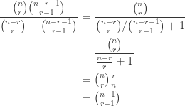
 ; note one may interpret an
  -tabloid as an ordered pair
  encoding the path of length 3 with edges
  and
and  . There is a
  acts on the set of set partitions of
  into
into  , where
  is the partition obtained from
  . So everything is in place to prove a version of the Erdős–Ko–Rado Theorem for perfect matchings. Update. I am grateful to Ehud for pointing out that this has
  . Perhaps, one day, this will be explained by defining the symmetric group as a group of automorphisms of a vector space over the field with one element. The analogue of the permutation module
  is that the maximum number of
  for
for  , where the
  -dimensional subspaces of
  . Thus the maximum is attained by taking all the subspaces containing a fixed line, in precise analogy with the case for sets. (Note also that if
  then any two
  is to
is to  where
where  is to
is to  .) Chapter 13 of his book has, I think, exactly what we need to prove the analogue of the lemma above. Update: I also just noticed that Section 8.6 of Harmonic analysis on finite groups by Ceccherini-Silberstein, Scarabotti and Tolli, titled ‘The
  where
where  is the maximal parabolic subgroup stabilising a chosen
  -dimensional subspace.
 and let
  be the permutation module of
  , let
, let  be the map sending a subspace to the formal linear combination of all
  -Specht module
  is then the intersection of the kernels of all the
  for
for  . Moreover if we set
 and
and  and
and  for
for  .
. .
. for
for  . An arbitrary
  in
in 
 and
and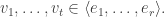
 such subspaces. Taking
  we get the result.
  when
when  and
and  when
when  by computer calculations. Note also that the
  counts, up to a power of
  , in good analogy with the symmetric group case. But it seems some careful analysis of reduced row-echelon forms (like the argument for the degree of
  .
. , and it is
 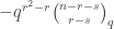 . Putting this into Hoffman’s bound and using that the subspaces graph is regular of degree
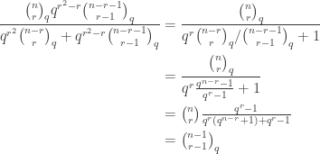
 on a vector space
  and
and  . In particular the actions of
 ,
,  and
and  be finite groups with
  . Then, for each
  , we have
 with
with  acting on the left on
  acting on the right, diagonally on each of the
  and
and  then one joint orbit is
 ; a little thought shows that the stabiliser of
  is
is
 : even though we are working in
  , it is not the case that the stabiliser factors as
  .
. rather than the formally correct
  .
. .
. where
where  is the subgroup of those
  fixing setwise the orbit
  . Moreover
  -modules
  .
. -modules
 as a
as a  -module in the second line and as a
  -module in the third line.
 is a normal subgroup of a permutation group
  then the orbits of
  . Then
  . This shows that
  and by symmetry equality holds.
 such that
  for some
  for some
  . These are equivalent conditions: take
  and use that the actions commute. Finally, identifying
  we see that
  . Since
  , as required.
 if and only if
  has a submodule isomorphic to
 ![\dim V = [K : L]\dim U](https://s0.wp.com/latex.php?latex=%5Cdim+V+%3D+%5BK+%3A+L%5D%5Cdim+U&bg=ffffff&fg=333333&s=0&c=20201002) . In this case we take
. In this case we take  -module
  .
. for induction on the left, we can state the following corollary with left- and right-actions.
 is a left
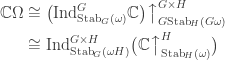
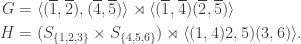
 and
and 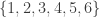 that respect the blocks
  ,
,  ,
,  ,
,  shown by the rooted trees in the graph below. The matching
  .
.
 and both
 . This is shown graphically below.
 . On the other hand, the permutation
  cannot be undone by a permutation in
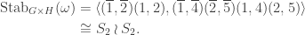
 .
.