
… aka Regressionizer demo
Introduction
This blog post provides examples of specifying different regression workflows using the class Regressionizer of the Python package “Regressionizer”, [AAp1].
The primary focus of Regressionizer is Quantile Regression (QR), [RK1, RK2]. It closely follows the monadic pipeline design explained in detail in the document “A monad for Quantile Regression workflows”, [AA1].
For introduction and overview of Quantile Regression see the video “Boston useR! QuantileRegression Workflows 2019-04-18”.
Summary of Regressionizer features
- The class
Regressionizerfacilitates rapid specifications of regressions workflows.- To quickly specify:
- data rescaling and summary
- regression computations
- outliers finding
- conditional Cumulative Distribution Functions (CDFs) reconstruction
- plotting of data, fits, residual errors, outliers, CDFs
- To quickly specify:
Regressionizerworks with data frames, numpy arrays, lists of numbers, and lists of numeric pairs.
Details and arguments
- The curves computed with Quantile Regression are called regression quantiles.
Regressionizerhas three regression methods:quantile_regressionquantile_regression_fitleast_squares_fit
- The regression quantiles computed with the methods
quantile_regressionandquantile_regression_fitcorrespond to probabilities specified with the argumentprobs. - The method
quantile_regressioncomputes fits using a B-spline functions basis.- The basis is specified with the arguments
knotsandorder. orderis 3 by default.
- The basis is specified with the arguments
- The methods
quantile_regession_fitandleast_squares_fituse lists of basis functions to fit with specified with the argumentfuncs.
Workflows flowchart
The following flowchart summarizes the workflows that are supported by Regressionizer:

Previous work
Roger Koenker implemented the R package “quantreg”, [RKp1]. Anton Antonov implemented the R package “QRMon-R” for the specification of monadic pipelines for doing QR, [AAp1].
Several Wolfram Language (aka Mathematica) packages are implemented by Anton Antonov, see [AAp1, AAp2, AAf1].
Remark: The paclets at the Wolfram Language Paclet Repository were initially Mathematica packages hosted at GitHub. The Wolfram Function Repository function QuantileRegression, [AAf1] does only B-spline fitting.
Setup
Load the “Regressionizer” and other “standard” packages:
from Regressionizer import *

import numpy as np
import plotly.express as px
import plotly.graph_objects as go
template='plotly'
Generate input data
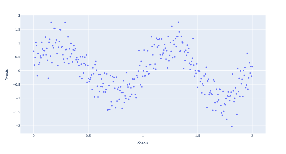
Generate random data:
np.random.seed(0)
x = np.linspace(0, 2, 300)
y = np.sin(2 * np.pi * x) + np.random.normal(0, 0.4, x.shape)
data = np.column_stack((x, y))
Plot the generated data:
fig = px.scatter(x=data[:, 0], y=data[:, 1], labels={'x': 'X-axis', 'y': 'Y-axis'}, template=template, width = 800, height = 600)
fig.show()
Fit given functions
Define a list of functions:
funcs = [lambda x: 1, lambda x: x, lambda x: np.cos(x), lambda x: np.cos(3 * x), lambda x: np.cos(6 * x)]
def chebyshev_t_polynomials(n):
    if n == 0:
        return lambda x: 1
    elif n == 1:
        return lambda x: x
    else:
        T0 = lambda x: 1
        T1 = lambda x: x
        for i in range(2, n + 1):
            Tn = lambda x, T0=T0, T1=T1: 2 * x * T1(x) - T0(x)
            T0, T1 = T1, Tn
        return Tn

chebyshev_polynomials = [chebyshev_t_polynomials(i) for i in range(10)]
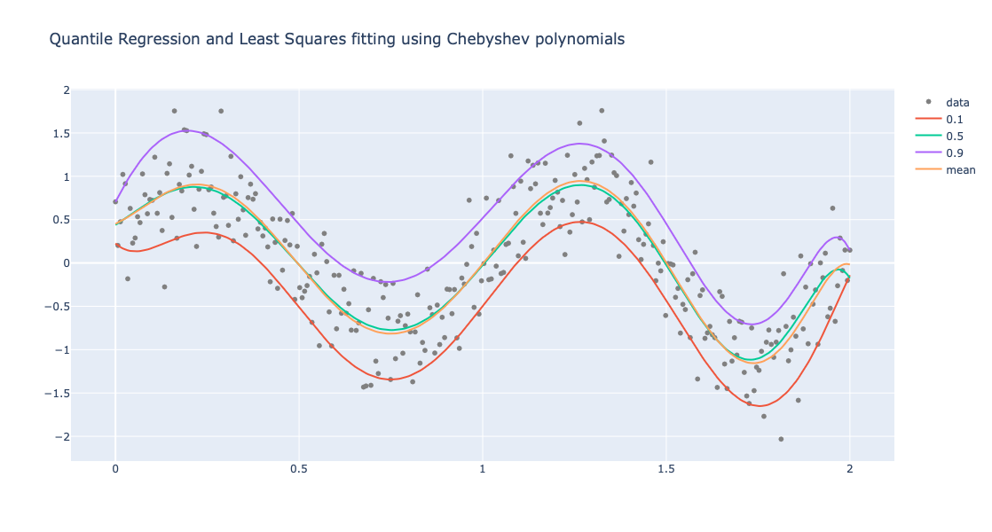
Define regression quantile probabilities:
probs = [0.1, 0.5, 0.9]
Perform Quantile Regression and (non-linear) Least Squares Fit:
obj2 = (
    Regressionizer(data)
    .echo_data_summary()
    .quantile_regression_fit(funcs=chebyshev_polynomials, probs=probs)
    .least_squares_fit(funcs=chebyshev_polynomials)
    .plot(title = "Quantile Regression and Least Squares fitting using Chebyshev polynomials", template=template)
)
Statistic    Regressor | Value
------------ --------------------
min                 0.0 | -2.0324132316043735
25%                 0.5 | -0.6063257640389526
median              1.0 | -0.0042185202753221695
75%                 1.5 | 0.6300535444986601
max                 2.0 | 1.757964402499859
Plot the obtained regression quantilies and least squares fit:
obj2.take_value().show()
Fit B-splines
Instead of coming-up with basis functions we can use B-spline basis:
obj = Regressionizer(data).quantile_regression(knots=8, probs=[0.2, 0.5, 0.8]).plot(title="B-splines fit", template=template)
Show the obtained plot:
obj.take_value().show()

Here is a dictionary of the found regression quantiles:
obj.take_regression_quantiles()
{0.2: <function QuantileRegression.QuantileRegression._make_combined_function.<locals>.<lambda>(x)>,
 0.5: <function QuantileRegression.QuantileRegression._make_combined_function.<locals>.<lambda>(x)>,
 0.8: <function QuantileRegression.QuantileRegression._make_combined_function.<locals>.<lambda>(x)>}
Weather temperature data
Load weather data:
import pandas as pd

url = "https://raw.githubusercontent.com/antononcube/MathematicaVsR/master/Data/MathematicaVsR-Data-Atlanta-GA-USA-Temperature.csv"
dfTemperature = pd.read_csv(url)
dfTemperature['DateObject'] = pd.to_datetime(dfTemperature['Date'], format='%Y-%m-%d')
dfTemperature = dfTemperature[(dfTemperature['DateObject'].dt.year >= 2020) & (dfTemperature['DateObject'].dt.year <= 2023)]
dfTemperature
| Date | AbsoluteTime | Temperature | DateObject | |
|---|---|---|---|---|
| 2555 | 2020-01-01 | 3786825600 | 7.56 | 2020-01-01 |
| 2556 | 2020-01-02 | 3786912000 | 7.28 | 2020-01-02 |
| 2557 | 2020-01-03 | 3786998400 | 12.28 | 2020-01-03 |
| 2558 | 2020-01-04 | 3787084800 | 12.78 | 2020-01-04 |
| 2559 | 2020-01-05 | 3787171200 | 4.83 | 2020-01-05 |
| … | … | … | … | … |
| 4011 | 2023-12-27 | 3912624000 | 11.67 | 2023-12-27 |
| 4012 | 2023-12-28 | 3912710400 | 7.44 | 2023-12-28 |
| 4013 | 2023-12-29 | 3912796800 | 3.78 | 2023-12-29 |
| 4014 | 2023-12-30 | 3912883200 | 4.83 | 2023-12-30 |
| 4015 | 2023-12-31 | 3912969600 | 1.17 | 2023-12-31 |
1461 rows × 4 columns
Convert to “numpy” array:
temp_data = dfTemperature[['AbsoluteTime', 'Temperature']].to_numpy()
temp_data.shape
(1461, 2)
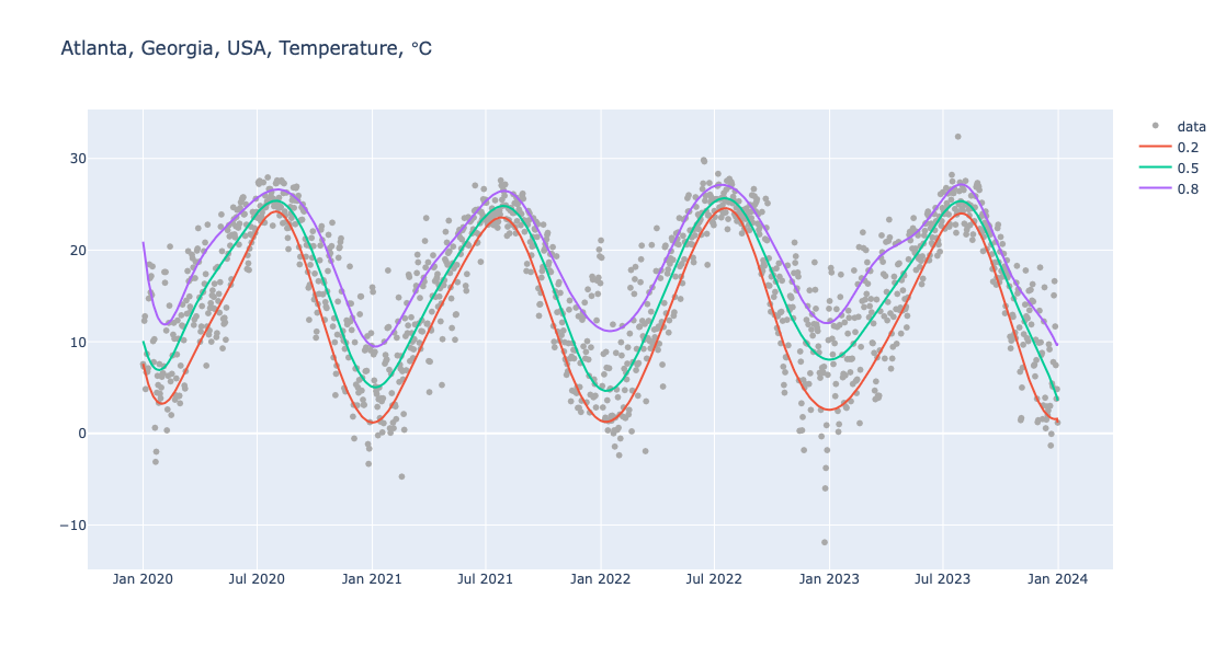
Here is pipeline for Quantile Regression computation and making of a corresponding plot:
obj = (
    Regressionizer(temp_data)
    .echo_data_summary()
    .quantile_regression(knots=20, probs=[0.2, 0.5, 0.8])
    .date_list_plot(title="Atlanta, Georgia, USA, Temperature, ℃", template=template, data_color="darkgray", width = 1200)
)
Statistic    Regressor | Value
------------ --------------------
min          3786825600.0 |     -11.89
25%          3818361600.0 |      10.06
median       3849897600.0 |      16.94
75%          3881433600.0 |      22.56
max          3912969600.0 |      32.39
Show the obtained plot:
obj.take_value().show()
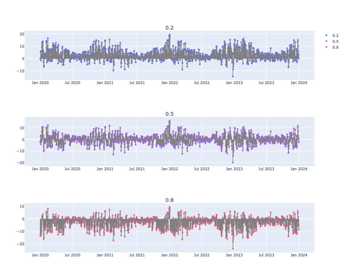
Fitting errors
Errors
Here the absolute fitting errors are computed and the average is for each is computed:
{ k : np.mean(np.array(d)[:,1]) for k, d in obj.errors(relative_errors=False).take_value().items() }
{0.2: 3.331223347420249, 0.5: 0.020191754857989016, 0.8: -3.3960272281557753}
Error plots
Here we give the fitting errors (residuals) for the regression quantiles found and plotted above:
obj.error_plots(relative_errors=False, date_plot=True, template=template, width=1200, height=300).take_value().show()
Outliers
One way to find contextual outliers in time series is to find regression quantiles at low- and high enough probabilities, and then select the points “outside” of those curves:
obj = (
    Regressionizer(temp_data)
    .quantile_regression(knots=20, probs=[0.01,  0.99], order=3)
    .outliers()
)

obj.take_value()
{'bottom': [array([ 3.7885536e+09, -3.1100000e+00]),
  array([3.7919232e+09, 3.2800000e+00]),
  array([3.795552e+09, 7.390000e+00]),
  array([3.7977984e+09, 9.2800000e+00]),
  array([3.7982304e+09, 1.0220000e+01]),
  array([3.8068704e+09, 2.0110000e+01]),
  array([3.8097216e+09, 1.2390000e+01]),
  array([ 3.8225088e+09, -4.7200000e+00]),
  array([3.8298528e+09, 1.0220000e+01]),
  array([3.8333952e+09, 1.8720000e+01]),
  array([3.8458368e+09, 3.5000000e+00]),
  array([ 3.8524896e+09, -2.3900000e+00])],
 'top': [array([3.7944288e+09, 2.2390000e+01]),
  array([3.802896e+09, 2.756000e+01]),
  array([3.8040192e+09, 2.7940000e+01]),
  array([3.8129184e+09, 2.3000000e+01]),
  array([3.814128e+09, 2.128000e+01]),
  array([3.820608e+09, 1.778000e+01]),
  array([3.8258784e+09, 2.3500000e+01]),
  array([3.8326176e+09, 2.7060000e+01]),
  array([3.839184e+09, 2.617000e+01]),
  array([3.8420352e+09, 2.2780000e+01]),
  array([3.8641536e+09, 2.9830000e+01]),
  array([3.8727072e+09, 2.5610000e+01]),
  array([3.8816928e+09, 1.8060000e+01])]}
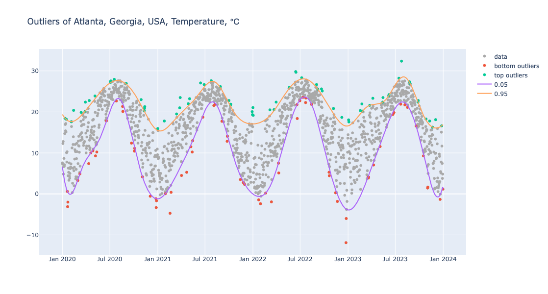
Here we plot the outliers (using a “narrower band” than above):
obj = (
    Regressionizer(temp_data)
    .quantile_regression(knots=20, probs=[0.05,  0.95], order=3)
    .outliers_plot(
        title="Outliers of Atlanta, Georgia, USA, Temperature, ℃",
        data_color="darkgray",
        date_plot=True,
        template=template,
        width = 1200)
)

obj.take_value().show()
Conditional CDF
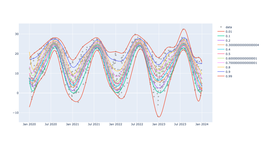
Here is a list of probabilities to be used to reconstruct Cumulative Distribution Functions (CDFs):
probs = np.sort(np.concatenate((np.arange(0.1, 1.0, 0.1), [0.01, 0.99])))
probs
array([0.01, 0.1 , 0.2 , 0.3 , 0.4 , 0.5 , 0.6 , 0.7 , 0.8 , 0.9 , 0.99])
Here we find the regression quantiles for those probabilities:
obj=(
    Regressionizer(temp_data)
    .quantile_regression(knots=20,probs=probs)
    .date_list_plot(template=template, data_color="darkgray", width=1200)
    )
Here we show the plot obtained above:
obj.take_value().show()
Get CDF function
Here we take a date in ISO format and convert to number of seconds since 1900-01-01:
from datetime import datetime

iso_date = "2022-01-01"
date_object = datetime.fromisoformat(iso_date)
epoch = datetime(1900, 1, 1)

focusPoint = int((date_object - epoch).total_seconds())
print(focusPoint)
3849984000
Here the conditional CDF at that date is computed:
aCDFs = obj.conditional_cdf(focusPoint).take_value()
aCDFs
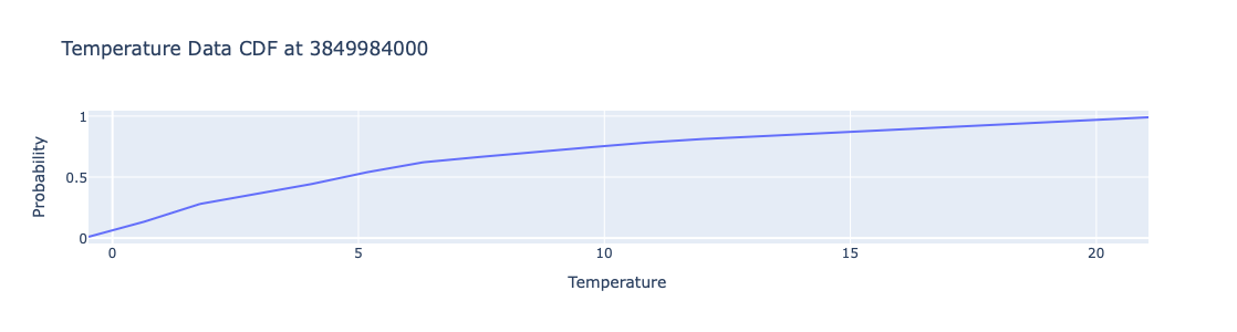
{3849984000: <scipy.interpolate._interpolate.interp1d at 0x135c2c460>}
Plot the obtained CDF function:
xs = np.linspace(obj.take_regression_quantiles()[0.01](focusPoint), obj.take_regression_quantiles()[0.99](focusPoint), 20)
cdf_values = [aCDFs[focusPoint](x) for x in xs]

fig = go.Figure(data=[go.Scatter(x=xs, y=cdf_values, mode='lines')])
# Update layout
fig.update_layout(
    title='Temperature Data CDF at ' + str(focusPoint),
    xaxis_title='Temperature',
    yaxis_title='Probability',
    template=template,
    legend=dict(title='Legend'),
    height=300,
    width=800
)
fig.show()
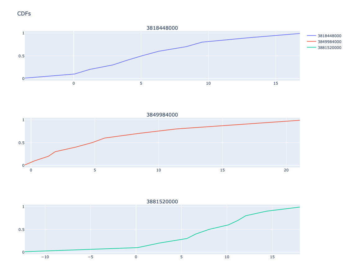
Plot multiple CDFs
Here are few dates converted into number of seconds since 1990-01-01:
pointsForCDFs = [focusPoint + i * 365 * 24 * 3600 for i in range(-1,2)]
pointsForCDFs
[3818448000, 3849984000, 3881520000]
Here are the plots of CDF at those dates:
obj.conditional_cdf_plot(pointsForCDFs, title = 'CDFs', template=template).take_value().show()
References
Articles, books
[RK1] Roger Koenker, Quantile Regression, Cambridge University Press, 2005.
[RK2] Roger Koenker, “Quantile Regression in R: a vignette”, (2006), CRAN.
[AA1] Anton Antonov, “A monad for Quantile Regression workflows”, (2018), MathematicaForPrediction at GitHub.
Packages, paclets
[AAp1] Anton Antonov, Quantile Regression Python package, (2024), GitHub/antononcube.
[AAp2] Anton Antonov, QRMon-R, (2019), GitHub/antononcube.
[AAp3] Anton Antonov, Quantile Regression WL paclet, (2014-2023), GitHub/antononcube.
[AAp4] Anton Antonov, Monadic Quantile Regression WL paclet, (2018-2024), GitHub/antononcube.
[AAf1] Anton Antonov, QuantileRegression, (2019), Wolfram Function Repository.
[RKp1] Roger Koenker, quantreg, CRAN.
Repositories
[AAr1] Anton Antonov, DSL::English::QuantileRegressionWorkflows in Raku, (2020), GitHub/antononcube.
Videos
[AAv1] Anton Antonov, “Boston useR! QuantileRegression Workflows 2019-04-18”, (2019), Anton Antonov at YouTube.
[AAv2] Anton Antonov, “useR! 2020: How to simplify Machine Learning workflows specifications”, (2020), R Consortium at YouTube.
