Jacobian Method

The Jacobian Method, also known as the Jacobi Iterative Method, is a fundamental algorithm used to solve systems of linear equations. It is useful when dealing with large systems where direct methods (like Gaussian elimination) are computationally expensive.

• The Jacobian Method works by breaking down a complex set of equations into simpler parts, making it easier to approximate the solutions.
• The Jacobian method leverages the properties of matrices to find solutions efficiently.

Here's a simple way to understand it:

Basics of Jacobian Method

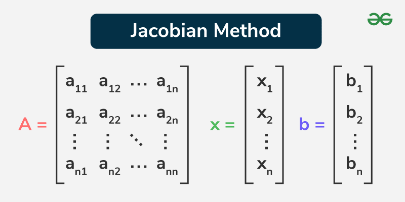
The method is used to solve a system of linear equations of the form:

Ax = b

Where A is a square matrix, x is the vector of unknowns, and b is the right-hand side vector.

The Jacobi Method decomposes the matrix A into its diagonal component D and the remainder R, such that:

A = D + R

The system of equations can then be rewritten as:

Dx = b − Rx

The iterative formula for the Jacobi Method is:

x^k+1 = D⁻¹(b − Rx^k)

Where x^k is the approximation of the solution at the k^th iteration.

Jacobi Iterative Implementation of Jacobian Method

The Jacobi iterative method is a specific implementation of the Jacobian method. It assumes that the system of linear equations can be written in the form Ax = b, where A is the coefficient matrix, x is the vector of unknown variables, and b is the vector of constants. The Jacobi method proceeds as follows:

• Assumption 1: The system of linear equations has a unique solution.
• Assumption 2: The coefficient matrix A has no zeros on its main diagonal.
• Assumption 3: The system is diagonally doominant( i.e., the absolute value of the diagonal elemnet in each row must be greater than or equal to the sum of the absolute values of the other elements in that row.)

Steps for Jacobi Iterative Method

We can use the following steps:

1. Check if the equations are idagonally dominant: if not rearrage the equations to make it diagonally dominant.
   For example, in the first equation: ∣a₁₁∣ ≥ ∣a₁₂∣ + ∣a₁₃∣, where a₁₁ is the coeffiecient of x, a₁₂ is the coeffiecient of y, and a₁₃ is the coeffiecient of z.
2. Rewrite the system of linear equations in the form: x_i = (b_i - ∑_{j≠i} a_{ij} x_j) / a_{ii}
3. Make an initial guess of the solution, x⁽⁰⁾ = (x₁⁽⁰⁾, x₂⁽⁰⁾, ..., x_n⁽⁰⁾).
4. Compute the first approximation, x⁽¹⁾, by substituting the initial guess into the rewritten equations.
5. Repeat step 3, using the previous approximation to compute the next approximation, until the desired accuracy is achieved.

Let's consider an example for better understanding:

Example : Consider the system of linear equations:

• 2x + y + z = 6
• x + 3y - z = 0
• -x + y + 2z = 3

Checking if the equations are diagonally dominant:

∣2∣ ≥ ∣1∣ + ∣1∣ = 2- true
∣3∣ ≥ ∣1∣ + ∣-1∣ = 2- true
∣2∣ ≥ ∣-1∣ + ∣1∣ = 2- true

Rewriting the system in the Jacobi form, we get:

x = (6 - y - z) / 2
y = (0 - x + z) / 3
z = (3 + x - y) / 2

Starting with the initial guess , the first approximation is:

Iteration 1: with p⁽⁰⁾ = (0, 0, 0)

x⁽¹⁾ = (6 - 0 - 0) / 2 = 3
y⁽¹⁾ = (0 - 0 + 0) / 3 = 0
z⁽¹⁾ = (3 + 0 - 0) / 2 = 1.5

Continuing the iterations, we obtain the following approximations:

Iteration 2: with p⁽¹⁾ = (3, 0, 1.5)

x⁽²⁾ = (6 − 0 − 1.5) / 2 = 2.25
y⁽²⁾ = (−3 + 1.5) / 3 = −0.5
z⁽²⁾ = (3 + 3 − 0) / 2 = 3

Iteration 3: with p⁽²⁾ = (2.25, -0.5, 3)

x⁽³⁾ = (6 + 0.5 − 3) / 2 = 1.75
y⁽³⁾ = (−2.25 + 3) / 3 = 0.25
z⁽³⁾ = (3 + 2.25 + 0.5) / 2 = 2.875

Iteration 4: with p⁽³⁾ = (1.75, 0.25, 2.875)

x⁽⁴⁾ = (6 - 0.25 - 2.875) / 2 = 1.4375
y⁽⁴⁾ = (0 - 1.75 + 2.875) / 3 = 0.375
z⁽⁴⁾ = (3 + 1.75 - 0.25) / 2 = 2.25

The values are converging slowly.

Therfore after 4 iterations we got: x ≈ 1.75, y ≈ 0.25, z ≈ 2.875.

After more iterations, you'll get a solution with more precision.

Jacobian Method in Matrix Form

Let the system of linear equations be Ax = b, where A is the coefficient matrix, x is the vector of unknown variables, and b is the vector of constants.

\begin{array}{cccccc}a_{11} x_1^{(k+1)} & + & a_{12} x_2^{(k)} & + \cdots + & a_{1n} x_n^{(k)} & = b_1 \\a_{21} x_1^{(k)} & + & a_{22} x_2^{(k+1)} & + \cdots + & a_{2n} x_n^{(k)} & = b_2 \\\vdots & & \vdots & & \vdots & \vdots \\a_{n1} x_1^{(k)} & + & a_{n2} x_2^{(k)} & + \cdots + & a_{nn} x_n^{(k+1)} & = b_n\end{array}

We can decompose the matrix A into three parts:

A = D + L + U

Where D is the diagonal matrix, L is the lower triangular matrix, and U is the upper triangular matrix.

\begin{bmatrix}a_{11} & 0 & \cdots & 0 \\0 & a_{22} & \cdots & 0 \\\vdots & \vdots & \ddots & \vdots \\0 & 0 & \cdots & a_{nn}\end{bmatrix}\begin{bmatrix}x_1^{(k+1)} \\x_2^{(k+1)} \\\vdots \\x_n^{(k+1)}\end{bmatrix}+\begin{bmatrix}0 & a_{12} & \cdots & a_{1n} \\a_{21} & 0 & \cdots & \vdots \\\vdots & \vdots & \ddots & \vdots \\a_{n1} & \cdots & a_{n,n-1} & 0\end{bmatrix}\begin{bmatrix}x_1^{(k)} \\x_2^{(k)} \\\vdots \\x_n^{(k)}\end{bmatrix}=\begin{bmatrix}b_1 \\b_2 \\\vdots \\b_n\end{bmatrix}

The Jacobi iteration can then be written as:

x^(k+1) = D^(-1) (b - (L + U)x^(k))

Where x^(k) and x^(k+1) are the kth and (k+1)^th approximations of the solution, respectively.

The element-based formula for the Jacobi method can be written as:

x_i^(k+1) = (b_i - ∑_{j≠i} a_{ij} x_j^{(k)}) / a_{ii}

This formula shows how the (k+1)^th approximation of the i^th variable is computed using the k^th approximations of the other variables.

Jacobian vs Gauss-Seidel Method

The difference between Jacobian and Gauss-Seidel method is given below:

Related Articles

• Root Finding Algorithms
• Newton Raphson Method

Solved Examples on Jacobian Method

Question 1: Consider the system of linear equations:

4x + y − z = 3
2x + 5y + z = 9
x + y + 3z = 7​

Checking if the equations are diagonally dominant:

∣4∣ ≥ ∣1∣ + ∣-1∣ = 2- true
∣5∣ ≥ ∣2∣ + ∣1∣ = 3- true
∣3| ≥ ∣1∣ + ∣1∣ = 2- true

We can rewrite this system in the Jacobi form as:

x = (3 - y + z)/4
y = (9 - 2x - z)/5
z = (7 - x - y)/3

Starting with the initial guess p⁽⁰⁾=(0,0,0)

Iteration 1:

Substitute the initial guess into the Jacobi equations:

x⁽¹⁾ = (3 − 0 + 0)/ 4 ​= 0.75
y⁽¹⁾ = (9 − 0 − 0)/5​ = 1.8
z⁽¹⁾ = (7 − 0 − 0)/3​ = 2.3333

First approximation: p⁽¹⁾=(0.75, 1.8, 2.33)

Iteration 2:

Substitute the first approximation into the Jacobi equations:

x⁽²⁾ = (3 − 1.8 + 2.33)/ 4 ​= 0.8833
y⁽²⁾ = (9 − 2(0.75) − 2.33)/5​ = 1.033
z⁽²⁾ = (7 − 0.75 − 1.8)/3​ = 1.4833

Second approximation: x⁽²⁾=(0.8833, 1.033, 1.4833)

Iteration 3:

Substitute the second approximation into the Jacobi equations:

x⁽³⁾ = (3 − 1.033 + 1.4833)/ 4 ​= 0.8625
y⁽³⁾ = (9 − 2(0.8833) − 1.4833)/5​ = 1.1500
z⁽³⁾ = (7 − 0.8833 − 1.033)/3​ = 1.6944

The values are converging slowly.

Therfore after 3 terations we got: x ≈ 0.8625, y ≈ 1.1500, z ≈ 1.6944.

After more iterations, you'll get a solution with more precision.

Question 2: Consider the following system of linear equations:

3x + 2y - z = 7
2x - y + 4z = 13
x + 3y + 2z = 12

Checking if the equations are diagonally dominant:

∣3∣ ≥ ∣2∣ + ∣-1∣ = 3- true
∣-1∣ ≥ ∣2∣ + ∣4∣ = 6- false
∣2| ≥ ∣1∣ + ∣3∣ = 4 - false

Swapping the equations we get,

3x+2y−z=7(1)
x+3y+2z=12(2)
2x−y+4z=13(3)​

∣3∣ ≥ ∣2∣ + ∣-1∣ = 3- true
∣3 ≥ ∣1∣ + ∣2∣ = 3- true
∣4| ≥ ∣2∣ + ∣-1∣ = 3 - true

We can rewrite this system in the Jacobi form as:

x = (7−2y+z) / 3​
y = (12−x−2z) / 3​
z = (13−2x+y) / 4​

Let's start with the initial guess p⁽⁰⁾=(0,0,0)

Iteration 1: Substituting the initial guess into the Jacobi equations, we get:

x⁽¹⁾ = (7 - 2(0) + 0)/3 = 7/3 = 2.333
y⁽¹⁾= (12 - 0 + 2(0))/3 = 4
z⁽¹⁾= (13 - 2(0) + 0)/4 = 13/4 = 3.25

Therefore, the first approximation is p⁽¹⁾=(2.333, 4, 3.25)

Iteration 2: Substituting the first approximation into the Jacobi equations, we get:

x⁽²⁾ = (7 - 2(4) + 3.25)/3 = 0.75
y⁽²⁾= (12 - 2.333 + 2(3.25))/3 = 1.0556
z⁽²⁾= (13 - 2(2.333) + 4)/4 = 3.0833

Therefore, the second approximation is p⁽²⁾=(0.75, 1.0556, 3.0833)

Iteration 3: Substituting the second approximation into the Jacobi equations, we get:

x⁽³⁾ = (7 - 2(1.0556) + 3.0833)/3 = 2.6574
y⁽³⁾= (12 - 0.75 + 2(3.0833))/3 = 1.6945
z⁽³⁾= (13 - 2(0.75) + 1.0556)/4 = 3.1389

Iteration 4: Substituting the third approximation into the Jacobi equations, we get:

x⁽⁴⁾ = (7 - 2(1.6945) + 3.1389)/3 = 2.25
y⁽⁴⁾= (12 - 2.6574 + 2(3.1389))/3 = 1.0216
z⁽⁴⁾= (13 - 2(2.6574) + 1.6945)/4 = 2.3449

The values are converging slowly.

Therfore after 4 iterations we got: x ≈ 2.25, y ≈ 1.0216, z ≈ 2.3449.

After more iterations, you'll get a solution with more precision.