Line Chart in Matplotlib - Python

A line chart in Matplotlib is used to display data points connected by straight lines. It is commonly used to visualize trends, changes, or patterns in data over a sequence, such as days, months, or years. Line charts make it easy to compare values and observe how data changes over time.

Example: In the example below, we create a basic line chart to display the relationship between the x-axis and y-axis values using the plot() function.

import matplotlib.pyplot as plt

x = [1, 2, 3, 4, 5]
y = [2, 4, 3, 5, 7]
plt.plot(x, y)
plt.show()

Output

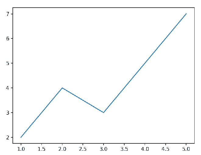
Explanation: plot() function creates a line chart by connecting the values in the x and y lists with straight lines. Finally, show() displays the chart on the screen.

Syntax

matplotlib.pyplot.plot(x, y, color=None, linestyle='-', linewidth=1, marker=None, label=None)

Parameters:

• x: Values to be displayed on the x-axis.
• y: Values to be displayed on the y-axis.
• color: Specifies the color of the line (for example, 'red', 'blue', 'green').
• linestyle: Defines the style of the line, such as solid ('-'), dashed ('--'), dotted (':'), or dash-dot ('-.').
• linewidth: Sets the thickness of the line.
• marker: Displays a marker at each data point (such as 'o', 's', '^', '*').
• label: Specifies a label for the plotted line, which is displayed when using legend().

Adding Labels and Title

Axis labels and a title make the chart easier to understand by describing the data being displayed.

import matplotlib.pyplot as plt
import numpy as np

x = np.array([1, 2, 3, 4])
y = x * 2

plt.plot(x, y)
plt.xlabel("X-axis")
plt.ylabel("Y-axis")
plt.title("Simple Line Plot with Labels")
plt.show()

Output

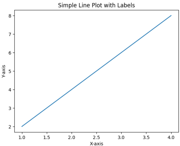
Explanation: xlabel(), ylabel() and title() functions add descriptive text to the x-axis, y-axis, and chart title.

Using Markers

Markers highlight individual data points on a line chart, making them easier to identify.

import matplotlib.pyplot as plt
import numpy as np

x = np.array([1, 2, 3, 4, 5])
y = [3, 6, 9, 12, 15]

plt.plot(x, y, marker='o', linestyle='-', label='Data Points')
plt.xlabel("X-axis")
plt.ylabel("Y-axis")
plt.title("Line Plot with Markers")
plt.legend()
plt.show()

Output

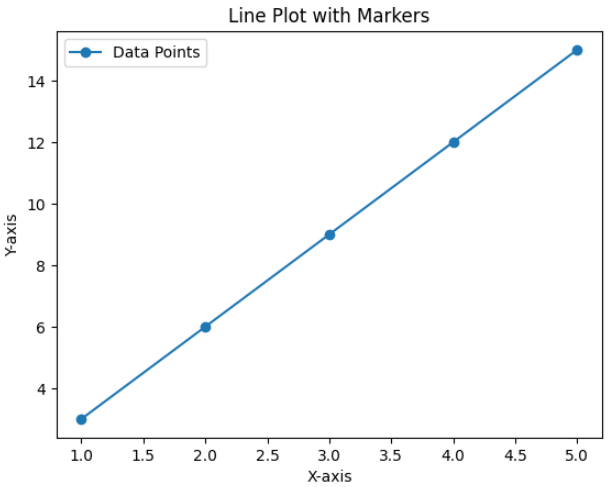
Explanation: marker parameter places a symbol at each data point while the line connects all points.

Adding a Grid

A grid improves readability by making it easier to compare data values with the axes.

import matplotlib.pyplot as plt

x = [1, 2, 3, 4]
y = [1, 4, 9, 16]

plt.plot(x, y)
plt.grid(True)
plt.xlabel("X-axis")
plt.ylabel("Y-axis")
plt.title("Line Plot with Grid")
plt.show()

Output

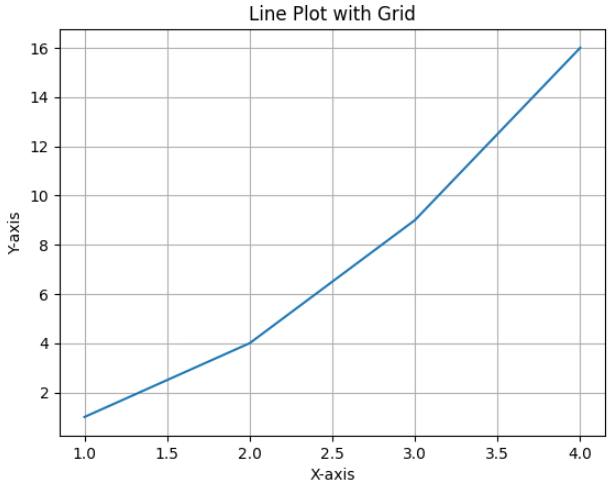
Explanation: grid(True) function displays horizontal and vertical grid lines on the plot.

Line Chart with Annotations

For adding annotations to a line chart you can use the annotate() function. This function allows you to display additional information such as the exact x and y values directly on the data points, improving clarity and data interpretation.

import matplotlib.pyplot as plt

x = [1, 2, 3, 4, 5]
y = [2, 4, 6, 8, 10]

plt.figure(figsize=(8, 6))
plt.plot(x, y, marker='o', linestyle='-')

for xi, yi in zip(x, y):
    plt.annotate(f'({xi}, {yi})',
                 (xi, yi),
                 textcoords="offset points",
                 xytext=(0, 10),
                 ha='center')

plt.title('Line Chart with Annotations')
plt.xlabel('X-axis')
plt.ylabel('Y-axis')
plt.grid(True)
plt.show()

Output

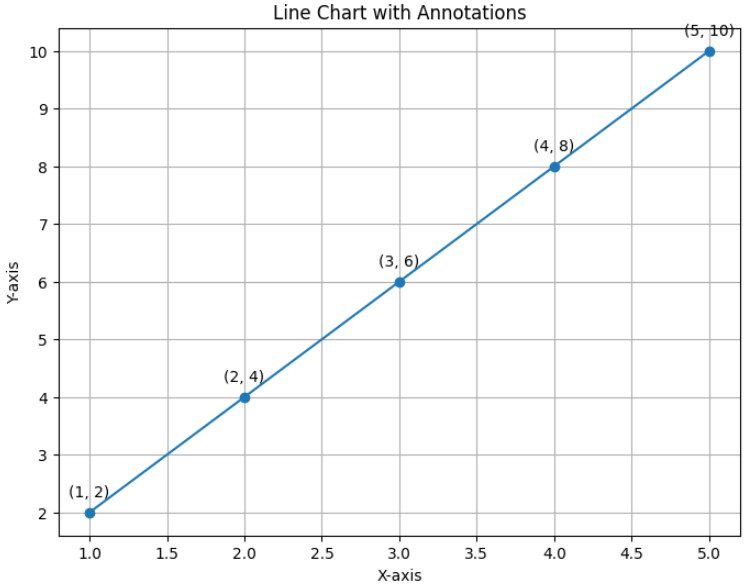
Explanation: annotate() function displays the coordinate value above each data point.

Multiple Line Charts

To create multiple line charts in separate containers you can use the figure() function. Each call to figure() generates a new plotting area, making it easier to visualize and compare different datasets independently.

import matplotlib.pyplot as plt
import numpy as np

x = np.array([1, 2, 3, 4])
y = x * 2

plt.plot(x, y)
plt.title("First Line Chart")
plt.show()

plt.figure()
x1 = [2, 4, 6, 8]
y1 = [3, 5, 7, 9]
plt.plot(x1, y1, '-.')
plt.title("Second Line Chart")
plt.show()

Output

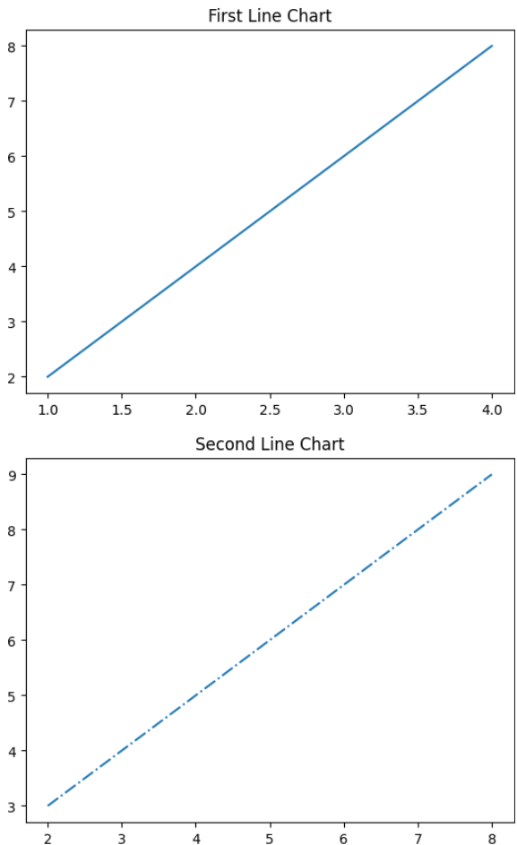
Explanation: figure() function creates a new figure so that each line chart is displayed separately.

Multiple Plots on Same Axis

To plot multiple lines on the same axis, you can call the plot() function multiple times before displaying the graph. This approach is useful for comparing different datasets within the same coordinate system.

import matplotlib.pyplot as plt
import numpy as np

x = np.array([1, 2, 3, 4])
y = x * 2

x1 = [2, 4, 6, 8]
y1 = [3, 5, 7, 9]

plt.plot(x, y, label='y = 2x')
plt.plot(x1, y1, '-.', label='Second Line')

plt.xlabel("X-axis data")
plt.ylabel("Y-axis data")
plt.title("Multiple Plots on Same Axis")
plt.legend()
plt.show()

Output

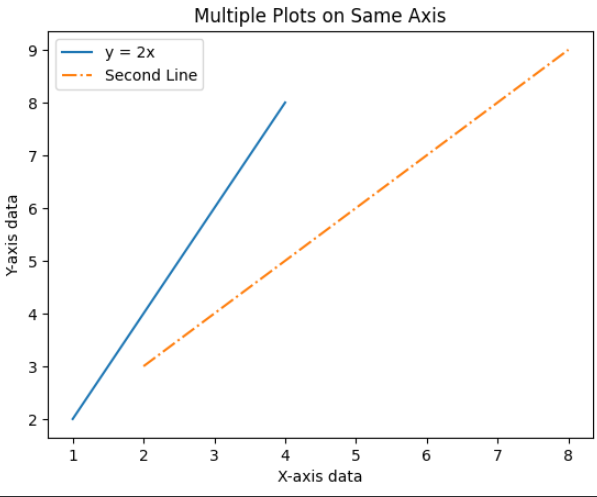
Explanation: Calling plot() multiple times before show() draws multiple lines on the same graph. The legend() function identifies each line.

Fill Area Between Two Lines

To fill the region between two line plots, you can use the fill_between() function. This function shades the area between two curves, helping visualize the difference or range between datasets.

import matplotlib.pyplot as plt
import numpy as np

x = np.array([1, 2, 3, 4])
y = x * 2
y1 = [3, 5, 7, 9]

plt.plot(x, y, label='y = 2x')
plt.plot(x, y1, '-.', label='y1')
plt.fill_between(x, y, y1, color='green', alpha=0.4)

plt.xlabel("X-axis data")
plt.ylabel("Y-axis data")
plt.title("Filled Area Between Two Lines")
plt.legend()
plt.show()

Output

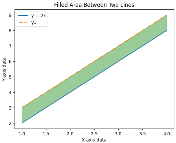
Explanation: fill_between() function shades the region enclosed by the two line plots.

Saving a Line Chart

Instead of displaying a plot you can save it as an image using the savefig() function.

import matplotlib.pyplot as plt

x = [1, 2, 3, 4]
y = [2, 4, 6, 8]

plt.plot(x, y)
plt.title("Saved Line Plot")
plt.savefig("line_plot.png")
plt.show()

Output

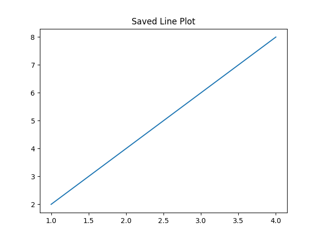
Explanation: savefig() function saves the current figure to an image file before or after displaying it.

Plotting Trigonometric Functions

Trigonometric functions such as sine, cosine and tangent can be visualized using plt.plot() by generating input values over a continuous range. The numpy.linspace() function creates evenly spaced values, allowing smooth and accurate curves.

import numpy as np
import matplotlib.pyplot as plt

x = np.linspace(0, 2 * np.pi, 100)
y_sin = np.sin(x)
y_cos = np.cos(x)

plt.plot(x, y_sin, label="sin(x)")
plt.plot(x, y_cos, label="cos(x)")
plt.xlabel("X values")
plt.ylabel("Function value")
plt.title("Trigonometric Functions")
plt.legend()
plt.show()

Output

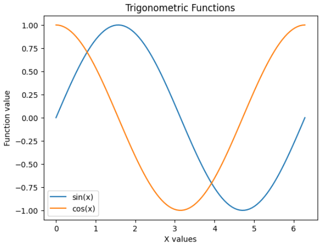
Explanation: linspace() function generates evenly spaced x-values, while sin() and cos() compute the corresponding y-values. Both functions are displayed on the same line chart for comparison.

You can download full code from here.