Broadcasting in NumPy allows us to perform arithmetic operations on arrays of different shapes without reshaping them. It automatically adjusts the smaller array to match the larger array's shape by replicating its values along the necessary dimensions. This makes element-wise operations more efficient by reducing memory usage and eliminating the need for loops.
Lets see an example:
Python
import numpy as np

a = np.array([[1, 2, 3], [4, 5, 6]])
x = 10
print(a + x)
Output[[11 12 13]
[14 15 16]]
Explanation:
- NumPy expands the scalar x to match the shape of array a.
- The operation a + x adds 10 to each element of a.
Working of Broadcasting in NumPy
Broadcasting applies specific rules to find whether two arrays can be aligned for operations or not that are:
- Check Dimensions: Ensure the arrays have the same number of dimensions or expandable dimensions.
- Dimension Padding: If arrays have different numbers of dimensions the smaller array is left-padded with ones.
- Shape Compatibility: Two dimensions are compatible if they are equal or one of them is 1.
If these conditions aren’t met NumPy will raise a ValueError. Lets see various examples for broadcasting below:
Example 1: Broadcasting a Scalar to a 1D Array
It creates a NumPy array arr with values [1, 2, 3] and adds a scalar value 1 to each element of the array using broadcasting.
Python
import numpy as np
arr = np.array([1, 2, 3])
res = arr + 1
print(res)
Example 2: Broadcasting a 1D Array to a 2D Array
This example shows how a 1D array a1 is added to a 2D array a2. NumPy automatically expands the 1D array along the rows of the 2D array to perform element-wise addition.
Python
import numpy as np

a = np.array([2, 4, 6])
b = np.array([[1, 3, 5], [7, 9, 11]])
res = a + b
print(res)
Output[[ 3 7 11]
[ 9 13 17]]
Explanation:
- a1 has shape (3,) and a2 has shape (2, 3).
- NumPy automatically repeats a1 across both rows of a2 so their shapes match.
- Then it adds elements position-wise: [1, 3, 5] + [2, 4, 6] = [3, 7, 11] and [7, 9, 11] + [2, 4, 6] = [9, 13, 17]
Example 3: Broadcasting in Conditional Operations
This example checks each age in the array and assigns "Adult" or "Minor" using np.where().
Python
import numpy as np

a = np.array([12, 24, 35, 45, 60, 72])
b = np.array(["Adult", "Minor"])
res = np.where(a > 18, b[0], b[1])
print(res)
Output['Minor' 'Adult' 'Adult' 'Adult' 'Adult' 'Adult']
Explanation:
- ages > 18 creates a Boolean array by checking every value at once (broadcasting).
- np.where() picks "Adult" for True and "Minor" for False without any loop.
- The result is an array labeling each age correctly.
Example 4: Using Broadcasting for Matrix Multiplication
In this example, each element of a 2D matrix is multiplied by the corresponding element in a broadcasted vector.
Python
import numpy as np
m = np.array([[1, 2], [3, 4]])
v = np.array([10, 20])
res = m * v
print(res)
Explanation:
- The vector v is broadcast across each row of m.
- Multiplication happens element-wise without loops.
- Result is a scaled version of the matrix.
Example 5: Scaling Data with Broadcasting
Consider a real-world scenario where we need to calculate the total calories in foods based on the amount of fats, proteins and carbohydrates. Each nutrient has a specific caloric value per gram.
- Fats: 9 calories per gram (CPG)
- Proteins: 4 CPG
- Carbohydrates: 4 CPG
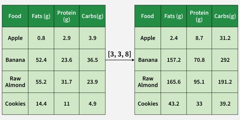 Scaling Data with Broadcasting
Left table shows the original data with food items and their respective grams of fats, proteins and carbs. The array [9, 4, 4] represents the caloric values per gram for fats, proteins and carbs respectively. This array is being broadcast to match the dimensions of the original data and arrow indicates the broadcasting operation.
- Broadcasting array is multiplied element-wise with each row of the original data.
- As a result right table shows the result of the multiplication where each cell represents the caloric contribution of that specific nutrient in the food item.
Python
import numpy as np

fd = np.array([ [0.8, 2.9, 3.9],
                [52.4, 23.6, 36.5],
                [55.2, 31.7, 23.9],
                [14.4, 11.0, 4.9] ])

cpg = np.array([9, 4, 4])
res = fd * cpg
print(res)
Output[[ 7.2 11.6 15.6]
[471.6 94.4 146. ]
[496.8 126.8 95.6]
[129.6 44. 19.6]]
Explanation:
- cpg (9, 4, 4) broadcasts across each row of fd.
- Each nutrient gram is multiplied by its calorie value.
- Result is a matrix showing calorie contribution from fats, proteins and carbs for each food item.
Example 6: Adjusting Temperature Data Across Multiple Locations
Suppose you have a 2D array representing daily temperature readings across multiple cities and you want to apply a correction factor to each city’s temperature data.
Python
import numpy as np

temp = np.array([ [30, 32, 34, 33, 31],
                  [25, 27, 29, 28, 26],
                  [20, 22, 24, 23, 21] ])

corr = np.array([1.5, -0.5, 2.0])
res = temp + corr[:, None]
print(res)
Output[[31.5 33.5 35.5 34.5 32.5]
[24.5 26.5 28.5 27.5 25.5]
[22. 24. 26. 25. 23. ]]
Explanation:
- corr[:, None] turns the 1D array into a column vector.
- NumPy broadcasts this vector down each row of temp.
- Each city’s temperatures get adjusted using its corresponding correction factor.
Example 7: Normalizing Image Data
Normalization is important in many real-world scenarios like image processing and machine learning because it:
- Centers data by subtracting the mean by ensuring features have zero mean.
- Scales data by dividing by the standard deviation by ensuring features have unit variance.
- Improves numerical stability and performance of algorithms like gradient descent.
Let's see how broadcasting simplifies normalization:
Python
import numpy as np

img = np.array([ [100, 120, 130],
                 [90, 110, 140],
                 [80, 100, 120] ])

m = img.mean(axis=0)
s = img.std(axis=0)
res = (img - m) / s
print(res)
Output[[ 1.22474487 1.22474487 0. ]
[ 0. 0. 1.22474487]
[-1.22474487 -1.22474487 -1.22474487]]
Explanation:
- m and s are 1D arrays (mean and std for each column).
- NumPy broadcasts them across all rows of img.
- (img - m) centers the data.
- Dividing by s scales it, giving the normalized values.
Example 8: Centering Data in Machine Learning
Centering data is an important step in many machine learning workflows. Broadcasting helps center the data efficiently by subtracting the mean from each feature. This example centers each feature by subtracting its mean using NumPy broadcasting.
Python
import numpy as np

data = np.array([ [10, 20],
                  [15, 25],
                  [20, 30] ])

m = data.mean(axis=0)
res = data - m
print(res)
Output[[-5. -5.]
[ 0. 0.]
[ 5. 5.]]
Explanation:
- m is a 1D array containing the mean of each column.
- NumPy broadcasts m across all rows.
- Subtracting it centers every feature around zero.
What is broadcasting in NumPy?
-
Creating videos from arrays
-
-
Stretching arrays with smaller shapes to perform operations
-
Explanation:
Broadcasting allows smaller arrays to fit larger ones during operations.
Which of the following is valid broadcasting?
-
-
[[1], [2], [3]] + [10, 20, 30]
-
-
Explanation:
NumPy allows scalar broadcasting (C) and shape matching broadcasting (B).
In NumPy broadcasting, when are two dimensions considered compatible?
-
Only when both dimensions are equal and greater than 1
-
Only when both dimensions are 1
-
When the dimensions are equal, or one of them is 1
-
When at least one dimension is greater than the other
Explanation:
In NumPy broadcasting, two dimensions are compatible if they are equal or if one of them is 1. NumPy virtually stretches the dimension with size 1 to match the other, allowing element-wise operations on different-shaped arrays.
Quiz Completed Successfully
Your Score : 2/3
Accuracy : 0%
Login to View Explanation
1/3
1/3
< Previous
Next >
Explore
Introduction
Creating NumPy Array
NumPy Array Manipulation