Histogram Equalization in OpenCV

Painting a vivid picture often hinges on the interplay of light and shadow within an image. Imagine having a tool that not only enhances those subtleties but breathes life into every pixel. Welcome to the world of ‘Histogram Equalization,’ an ingenious technique that transforms lackluster visuals into stunning masterpieces.

In this article, we embark on a journey through the vibrant realm of OpenCV’s Histogram Equalization, uncovering its power to revitalize images and amplify their visual impact.

What is a histogram image in OpenCV?

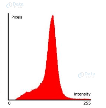
In OpenCV, a histogram image is a visual representation of the frequency distribution of pixel intensities within a grayscale image. Essentially, it provides insights into how different intensity values are distributed throughout the image. A histogram displays the range of pixel intensities on the x-axis and the frequency of each intensity value on the y-axis.

Histograms are valuable tools for image analysis and enhancement. They offer a comprehensive view of an image’s tonal distribution, helping us understand its contrast, brightness, and overall quality.

Histograms are widely used in various image processing tasks, including adjusting image levels, enhancing contrast, and performing operations like histogram equalization.

OpenCV provides functions to calculate and visualize histograms, making it easier to analyze and manipulate the intensity distribution of images. By studying a histogram image in OpenCV, you can gain insights into the underlying characteristics of an image and make informed decisions about how to enhance or modify it.

Keep in mind that our histogram includes many peaks, indicating that there are many pixels binned to each of the corresponding buckets. Our objective with histogram equalization is to distribute these pixels among buckets with fewer pixels binned to them.

This indicates that we are trying to apply a linear trend to our cumulative distribution function (CDF) mathematically.

Working of Histogram equalization in OpenCV

To achieve the spreading of intensity values over the entire range, histogram equalization converts one distribution of the provided histogram to another distribution (a distribution with a more uniform intensity value distribution).

The cumulative distribution function is used during remapping to produce the equalization effect.

The cumulative distribution H'(i) for the histogram H(i) is given by:

H'(i)=∑0≤j<iH(j)

The Histogram H’i must be normalized before the cumulative distribution function may be used for remapping. An image should have a maximum intensity value of 255. Following a straightforward remapping technique, intensity values for the equalized image are acquired.

equalized(x,y)=H'(src(x,y))

Illuminating Insights: Visualizing Image and Histogram with OpenCV

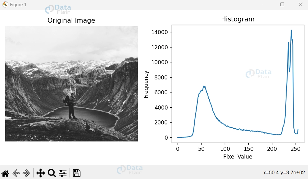
In the world of image manipulation, there exists a powerful duo that grants us unprecedented insights into the inner workings of visuals: the original image and its corresponding histogram. These two elements, when paired harmoniously, offer a glimpse into the distribution of pixel intensities, shedding light on the image’s tonal range, contrast, and more. In this exploration, we delve into the captivating realm of OpenCV, unravelling the process of displaying the original image side by side with its histogram graph using the creative prowess of Python’s Matplotlib.

Process Overview:

1. Load the Image: Begin by loading the grayscale image you wish to analyze. This serves as the canvas upon which the histogram’s story unfolds.

2. Histogram Calculation: Employ OpenCV’s `cv2.calcHist()` function to compute the histogram of the loaded image. This function calculates the frequency distribution of pixel intensities within the image.

3. Display Original Image: Set the stage by showcasing the original image on the left side. This allows for direct visual comparison with the histogram to follow.

4. Plot the Histogram: On the right side, craft the histogram graph using Matplotlib. With pixel values on the x-axis and their corresponding frequencies on the y-axis, the histogram paints a vivid picture of the image’s intensity distribution.

5. Present the Insights: By unveiling both the original image and its histogram, you gain unparalleled insights into the image’s tonal variations, contrast levels, and more.

Code Example:

import cv2
import numpy as np
import matplotlib.pyplot as plt

# Load the image
image = cv2.imread(r"C:\Users\satchit\Desktop\DataFlair\histogram equalization in OpenCV\beautiful-mountains.jpg", cv2.IMREAD_GRAYSCALE)

# Calculate the histogram
histogram = cv2.calcHist([image], [0], None, [256], [0, 256])

# Display the original image
plt.figure(figsize=(8, 4))
plt.subplot(1, 2, 1)
plt.imshow(cv2.cvtColor(image, cv2.COLOR_BGR2RGB))
plt.title('Original Image')
plt.axis('off')

# Display the histogram
plt.subplot(1, 2, 2)
plt.plot(histogram)
plt.title('Histogram')
plt.xlabel('Pixel Value')
plt.ylabel('Frequency')

# Show the plots
plt.tight_layout()
plt.show()

The synergy between an image and its histogram transcends mere visualization—it empowers us to comprehend the intricate dance of pixel intensities that form the essence of our visuals. By harnessing OpenCV’s capabilities and Matplotlib’s creative canvas, you are primed to unlock newfound depths of image analysis and manipulation.

Histogram Equalization in OpenCV

In the quest to transform lackluster images into vibrant masterpieces, the art of histogram equalization emerges as a pivotal technique. This process offers an enchanting way to enhance image contrast, reveal hidden details, and invigorate visual storytelling. Within the realm of OpenCV, this technique becomes even more accessible, thanks to its built-in functions designed to effortlessly breathe life into your images.

Algorithm:

The algorithm behind histogram equalization revolves around redistributing pixel intensities in an image to achieve a more balanced and appealing tonal distribution. This process involves calculating the Cumulative Distribution Function (CDF) of pixel intensities and mapping them to new values to spread them more evenly across the available range.

Working:

1. Compute Histogram: Calculate the histogram of the input image to understand the frequency distribution of pixel intensities.

2. Calculate CDF: Compute the CDF of the histogram to determine the cumulative probability of each intensity level.

3. Equalization Transformation: Utilize the CDF to transform the pixel intensities, ensuring a more uniform distribution across the entire intensity range.

Types of Histogram Equalization:

1. Global Histogram Equalization: Enhances overall image contrast by equalizing the entire image based on its global intensity distribution.

2. Local Histogram Equalization (CLAHE): Adapts equalization to smaller image regions, preventing over-amplification of noise and preserving local contrast.

cv2.equalizeHist() – Syntax and Parameters:

equalized_image = cv2.equalizeHist(image)

• Image: The grayscale image is to be equalized.
• Equalized_image: The resulting image after histogram equalization.

Code Example – Using cv2.equalizeHist():

import cv2
import numpy as np
import matplotlib.pyplot as plt
# Load the image
image = cv2.imread(r"C:\Users\satchit\Desktop\DataFlair\histogram equalization in OpenCV\beautiful-mountains.jpg", cv2.IMREAD_GRAYSCALE)
# Apply histogram equalization
equalized_image = cv2.equalizeHist(image)

# Display the original and equalized images
cv2.imshow('Original Image', image)
cv2.imshow('Equalized Image', equalized_image)
cv2.waitKey(0)
cv2.destroyAllWindows()

Original Image:

Equalized Image:

In this code, we load the grayscale image and apply histogram equalization using the cv2.equalizeHist() function. The resulting images showcase the transformative power of this technique, as the equalized image exhibits enhanced contrast and a more balanced tonal distribution.

From concept to implementation, histogram equalization in OpenCV holds the key to revitalizing your images, granting them the visual allure they truly deserve.

Adaptive Histogram Equalization (AHE) and Contrastive Limited Adaptive Equalization

Adaptive Histogram Equalization (AHE):

Adaptive Histogram Equalization (AHE) is an image processing technique used to enhance the contrast of an image by locally adjusting the intensity levels based on the histogram of small regions within the image. This technique is particularly effective in enhancing the contrast of images with varying illumination conditions.

Contrastive Limited Adaptive Equalization (CLAHE):

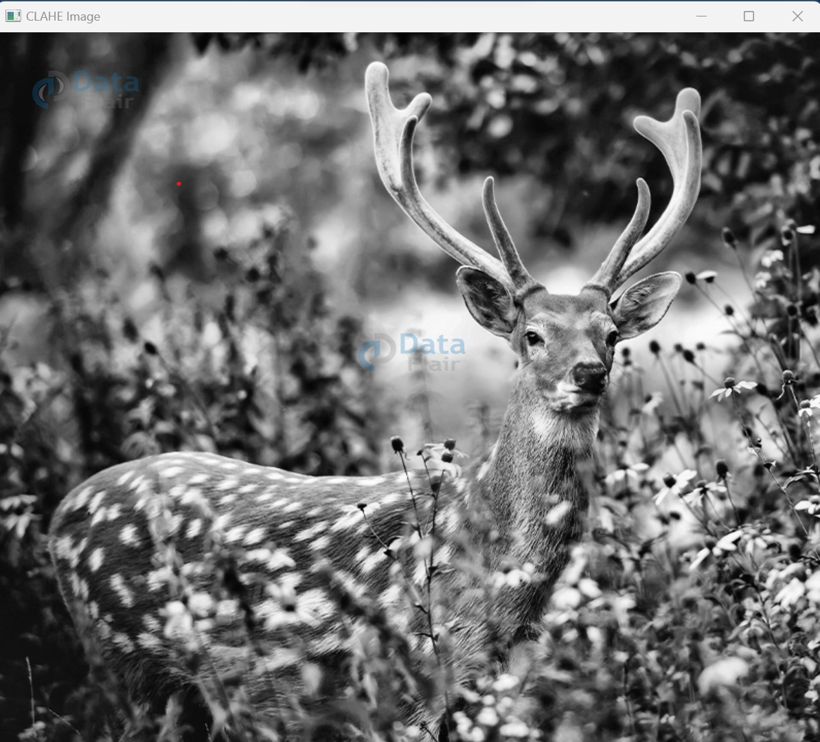
Contrastive Limited Adaptive Equalization (CLAHE) is an extension of AHE that addresses the problem of over-amplification of noise in regions with low contrast. CLAHE divides the image into small blocks, applies AHE to each block, and then limits the contrast enhancement by redistributing excess contrast from highly contrasted blocks to those with lower contrast.

Let’s use Python and the OpenCV library to demonstrate Adaptive Histogram Equalization (AHE) and Contrastive Limited Adaptive Equalization (CLAHE):

import cv2
import numpy as np

# Load an image
image = cv2.imread('input_image.jpg', cv2.IMREAD_GRAYSCALE)

# Apply Adaptive Histogram Equalization (AHE)
ahe = cv2.createCLAHE(clipLimit=2.0, tileGridSize=(8, 8))  # Clip limit and grid size can be adjusted
ahe_image = ahe.apply(image)

# Apply Contrastive Limited Adaptive Equalization (CLAHE)
clahe = cv2.createCLAHE(clipLimit=2.0, tileGridSize=(8, 8))
clahe_image = clahe.apply(image)

# Display the original, AHE, and CLAHE images
cv2.imshow('Original Image', image)
cv2.imshow('AHE Image', ahe_image)
cv2.imshow('CLAHE Image', clahe_image)
cv2.waitKey(0)
cv2.destroyAllWindows()

Original Image:

AHE Image:

CLAHE Image:

In this code, we first load an input grayscale image (‘input_image.jpg’). We then create instances of AHE and CLAHE using the `cv2.createCLAHE` function from the OpenCV library. The `clipLimit` parameter determines the extent of contrast limiting, and the `tileGridSize` parameter specifies the size of the local regions. You can adjust these parameters according to your preferences and the characteristics of the input image.

After applying AHE and CLAHE, we display the original, AHE-enhanced, and CLAHE-enhanced images using the `cv2.imshow` function. The `cv2.waitKey(0)` function waits for a key press before closing the image windows.

Please note that the effectiveness of AHE and CLAHE depends on various factors, including the nature of the input image and the parameter settings used. Experimentation and parameter tuning might be necessary to achieve the desired results.

Summary

In the realm of image enhancement, the art of histogram equalization emerges as a beacon of transformation, turning ordinary images into extraordinary visual narratives. With a profound understanding of the algorithm’s inner workings, we’ve explored how OpenCV effortlessly empowers us to weave magic into our images.

From calculating histograms and mapping pixel intensities to embracing global and local variations, histogram equalization offers a myriad of approaches to enhance image quality. By harnessing the cv2.equalizeHist() function, we’ve unveiled a gateway to effortlessly unleash the potential locked within our visuals.

In this journey, we’ve navigated the intricacies of histogram equalization, delving into its essence, its types, and its seamless integration into OpenCV. Armed with this knowledge, you are now poised to breathe life into images, illuminating hidden details and reviving the visual allure that captivates our senses.

As you embark on your image manipulation endeavors, remember that the power to craft enchanting visuals rests at your fingertips, thanks to the enchanting art of histogram equalization.