Working with Images in Python using Matplotlib

The fields of computer vision, medical imaging, and digital media all rely heavily on advances in image processing. Improving or gaining insight from digital pictures requires analysing, improving, and modifying them. This tutorial focuses on utilising the robust Matplotlib module in Python, which offers a full suite of tools for dealing with pictures.

Getting images to load and show up

Importing the Necessary Libraries

It’s important to import the appropriate libraries before getting started with image processing. In addition to NumPy and OpenCV, Matplotlib also provides a wide variety of tools and methods for manipulating visual data. Maintaining Python compatibility is also essential.

Take a look at this code snippet for an example of library import:

import matplotlib.pyplot as plott
import numpy as numpyy
from matplotlib.image import imread

Loading Images

The first step in dealing with pictures in Python is to import them from files. The imread function in Matplotlib makes it easy to load pictures saved in formats like JPEG and PNG. Successful picture loading requires familiarity with many image formats and the ability to convert between them.

A sample of Matplotlib code to load an image with the name “3d-plots-in-matplotlib.jpeg” is as follows:

from matplotlib.image import imread


image_path = '/content/3d-plots-in-matplotlib.jpeg' #This is the path of image


img = imread(image_path)

Viewing Figures

After an image is loaded, the imshow function in Matplotlib may be used to display it. The picture is plotted so you can see what’s within thanks to this feature. Image visualisation may be improved by modifying display settings like colormap and interpolation.

Take this sample of code for showing an image in Matplotlib as an example:

# Display image
plott.imshow(img)


# Customize display options
plott.imshow(img, cmap='gray', interpolation='nearest')

Transformation and Manipulation of Images in Matplotlib

Image Reduction and Enlargement

Image processing often involves actions like resizing and scaling pictures. The resize function in Matplotlib lets you modify an image’s width, height, and aspect ratio. This is helpful for tailoring photos to unique specifications or intended displays.

A sample of Matplotlib code to resize a picture is as follows:

import matplotlib.pyplot as plott
from skimage.transform import resize


# Define the desired height and width
changed_height = 300
changed_width = 400


# Resize image
resized_image = resize(img, (changed_height, changed_width))
plott.imshow(resized_image)

Cropping and Identifying Key Areas

There are times when you need to zero down on a very precise part of a picture. Selecting and extracting regions of interest (ROI) from a picture is made possible using Matplotlib’s slicing and indexing features. This opens the door to future investigation or focus on certain aspects.

Take the following Matplotlib code snippet as an example:

# Assuming the variables b1, b2, a1, and a2 are the coordinates of the cropping region
b1 = 100
b2 = 300
a1 = 200
a2 = 400


# Crop image
cropped_image = img[b1:b2, a1:a2]
plott.imshow(cropped_image)

Flipping and rotating images

In order to alter an image’s orientation or viewpoint, popular transformations include rotation and flipping. The rotate function in Matplotlib allows for the picture to be rotated in a variety of ways. Images may be flipped horizontally or vertically for mirrored effects or to get new insights.

To illustrate how to rotate an image using Matplotlib, consider the following code snippet:

# Rotate image
rotated_image = numpyy.rot90(img, k=1)  # 90-degree rotation
plott.imshow(rotated_image)

Enhancing and filtering images in Matplotlib

Incorporating Filters

Filters are essential in image processing since they alter the values of the pixels of a picture to get the desired result. Matplotlib has a number of filter functions that may be used to blur or sharpen pictures. Filters may be used to improve picture quality, get rid of unwanted noise, and get images ready for further research and visualisation.

Think about this Matplotlib code snippet for adding a Gaussian blur to an image:

from skimage.filters import gaussian


# Apply Gaussian filter to image
filtered_image = gaussian(img, sigma=2)
plott.imshow(filtered_image)

Making Changes to the Hue, Contrast, and Saturation

Brightness, contrast, and saturation adjustments may have a large influence on an image’s overall aesthetic appeal and readability. Matplotlib has methods to change these attributes, so you may tweak the necessary settings to make details in the picture more visible.

For instance, consider this Matplotlib code snippet for modifying the image’s hue, saturation, and brightness:

import matplotlib.pyplot as plott
from skimage import exposure


# Load the image
img = plott.imread('/content/3d-plots-in-matplotlib.jpeg')


# Adjust brightness, contrast, and saturation
brightness_factor = 1.2
contrast_factor = 1.5
saturation_factor = 1.3


# Adjust brightness using gamma correction
adjusted_img = exposure.adjust_gamma(img, brightness_factor)


# Adjust contrast
adjusted_img = exposure.rescale_intensity(adjusted_img, in_range='image', out_range=(0, 1))
adjusted_img = exposure.adjust_gamma(adjusted_img, 1 / contrast_factor)


# Adjust saturation
adjusted_img = exposure.adjust_gamma(adjusted_img, 1 / saturation_factor)


# Display the original and adjusted images
fig, axes = plott.subplots(1, 2, figsize=(10, 5))


axes[0].imshow(img)
axes[0].set_title('Original Image DataFlair')
axes[0].axis('off')


axes[1].imshow(adjusted_img)
axes[1].set_title('Adjusted Image DataFlair')
axes[1].axis('off')


plott.show()

This code uses the skimage method adjust_gamma() to tweak the image’s contrast. Next, we change the brightness using the rescale_intensity() method, and last, we tweak the saturation with another use to the adjust_gamma() function.

Matplotlib for Image Processing

Although Matplotlib isn’t designed primarily for image processing, its capabilities may be expanded to carry out simple picture alteration operations. We may display pictures in plots using the imshow() method that is provided by Matplotlib. NumPy arrays may also be used to change an image’s pixel values.

Image negative

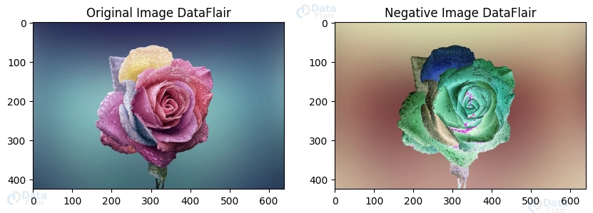
Let’s begin with a basic example of using Matplotlib to perform the image negative procedure on an image;

import matplotlib.pyplot as plott
import matplotlib.image as mpimg
import numpy as numpyy


# Load the image
image = mpimg.imread('/image2.jpg')


# Perform image negative
negative_image = 1 - image


# Display the original and negative images
plott.figure(figsize=(10, 5))
plott.subplot(1, 2, 1)
plott.imshow(image)
plott.title('Original Image DataFlair')


plott.subplot(1, 2, 2)
plott.imshow(negative_image)
plott.title('Negative Image DataFlair')


plott.show()

In this example, we use mpimg.imread() to load an image, and then we apply the image negative operations by reducing the value of each pixel by 1. Then, using plt.subplot() and plt.imshow(), we show both the positive and negative pictures side by side.

Modern Techniques for Image Processing in Matplotlib

While Matplotlib is capable of handling simple image processing, we may combine it with additional libraries like Scipy, OpenCV, or PIL (Python Imaging Library) to do more complex tasks. Let’s look at some sophisticated Scipy image processing methods.

Scipy to blur an image.

When decreasing noise or obscuring crucial information, blurring a picture may be helpful. To apply Gaussian blurring to pictures, Scipy offers the ndimage.gaussian_filter() method.

import matplotlib.pyplot as plott
import matplotlib.image as mpimg
import numpy as numpyy
from scipy.ndimage import gaussian_filter


# Load the image
image = mpimg.imread('/image2.jpg')


# Apply Gaussian blur with sigma=3
blurred_image = gaussian_filter(image, sigma=3)


# Display the original and blurred images
plott.figure(figsize=(10, 5))
plott.subplot(1, 2, 1)
plott.imshow(image)
plott.title('Original Image DataFlair')


plott.subplot(1, 2, 2)
plott.imshow(blurred_image)
plott.title('Blurred Image DataFlair')


plott.show()

To add Gaussian blurring to the picture in this example, we utilise the gaussian_filter() function from Scipy’s ndimage package. The sigma parameter regulates the level of blurring.

Scipy to Detect Image Edges

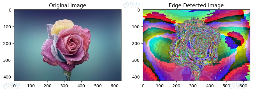
Edge detection is a key image processing method used to identify the borders and edges of objects in a picture. For edge detection, Scipy offers the ndimage.sobel() method.

import matplotlib.pyplot as plott
import matplotlib.image as mpimg
import numpy as numpyy
from scipy.ndimage import sobel


# Load the image
image = mpimg.imread('/image2.jpg')


# Apply edge detection using Sobel filter
edge_image = sobel(image)


# Display the original and edge-detected images
plott.figure(figsize=(10, 5))
plott.subplot(1, 2, 1)
plott.imshow(image)
plott.title('Original Image DataFlair')


plott.subplot(1, 2, 2)
plott.imshow(edge_image)
plott.title('Edge-Detected Image DataFlair')


plott.show()

In this example, edge detection is applied to the picture using the sobel() function from the ndimage module of Scipy. The gradient magnitude is calculated by the function, emphasising the edges of the picture.

Tones and Shades

The brightness, contrast, and saturation of a picture may be changed using tint, shade, and tone colour modification methods.

Image Shading

A picture is shaded by adding black or white to make it look darker or lighter. By modifying the pixel values, Matplotlib allows us to add shade.

import matplotlib.pyplot as plott
import matplotlib.image as mpimg
import numpy as numpyy


# Load the image
image = mpimg.imread('/image3.png')


# Define the shading factor (0.5 for lighter, 1.5 for darker)
shading_factor = 0.5


# Apply shading by adjusting pixel values
shaded_image = numpyy.clip(image * shading_factor, 0, 1)


# Display the original and shaded images
plott.figure(figsize=(10, 5))
plott.subplot(1, 2, 1)
plott.imshow(image)
plott.title('Original Image DataFlair')


plott.subplot(1, 2, 2)
plott.imshow(shaded_image)
plott.title('Shaded Image DataFlair')


plott.show()

In this illustration, we first establish a shading factor (for instance, 0.5 for lighter shading, 1.5 for deeper shading), and then we apply the shading by modifying the pixel values in accordance with the shading factor.

Image gradation

Toning involves changing an image’s saturation, giving it a desaturated or sepia tone. By changing the picture’s colour space to HSV and modifying the saturation channel, we may use Matplotlib to tone an image.

import matplotlib.pyplot as plott
import matplotlib.image as mpimg
import cv2
import numpy as numpyy


# Load the image
image = mpimg.imread('/image3.png')


# Convert the image to BGR format (required by cv2)
bgr_image = cv2.cvtColor(image, cv2.COLOR_RGB2BGR)


# Define the toning factor (0 for desaturated, 1 for original, 2 for sepia-toned)
toning_factor = 2


# Convert the image to LAB color space
lab_image = cv2.cvtColor(bgr_image, cv2.COLOR_BGR2Lab)


# Split the LAB image into L, A, and B channels
l_channel, a_channel, b_channel = cv2.split(lab_image)


# Multiply the A and B channels by the toning factor
a_channel = numpyy.clip(a_channel * toning_factor, 0, 255)
b_channel = numpyy.clip(b_channel * toning_factor, 0, 255)


# Merge the modified channels back into the LAB image
lab_toned_image = cv2.merge((l_channel, a_channel, b_channel))


# Convert the LAB image back to BGR color space
bgr_toned_image = cv2.cvtColor(lab_toned_image, cv2.COLOR_Lab2BGR)


# Convert the BGR image back to RGB format (required by matplotlib)
toned_image = cv2.cvtColor(bgr_toned_image, cv2.COLOR_BGR2RGB)


# Display the original and toned images
plott.figure(figsize=(10, 5))
plott.subplot(1, 2, 1)
plott.imshow(image)
plott.title('Original Image DataFlair')


plott.subplot(1, 2, 2)
plott.imshow(toned_image)
plott.title('Toned Image DataFlair')


plott.show()

The colorsys.rgb_to_hsv() function is used in this example to convert the picture to the HSV colour space. The picture is then returned to the RGB colour space using colorsys.hsv_to_rgb() after the saturation channel has been adjusted depending on the toning factor.

Image Export and Storage

Storing Pictures in a File

After finishing editing your pictures, you may wish to save them in files for further review or distribution. Matplotlib’s imsave function enables you to save pictures in a number of different file formats, including JPEG and PNG. The act of storing photographs in files preserves their longevity and makes them accessible in a variety of contexts.

Take the following Matplotlib code snippet as an example of how to save an image:

from matplotlib.image import imsave


imsave('processed_image.jpg', adjusted_img)

Saving Images for Publication or the Web

File size, resolution, and picture quality are all significant considerations when exporting photographs for use on the web or in print. Matplotlib gives you the option of exporting pictures in optimised formats like JPEG or PNG, allowing you to strike a compromise between these factors. Optimising photos for their intended use maximises visual quality while decreasing file size.

Take a look at this code snippet as an example of how to export a picture in JPEG format with a fixed compression level using Matplotlib:

from PIL import Image


# Convert the adjusted image to the PIL Image format
pil_image = Image.fromarray((adjusted_img * 255).astype(numpyy.uint8))


# Save the image in an optimized JPEG format with the desired quality
pil_image.save('optimized_image.jpg', format='JPEG', quality=90)

Conclusion

In conclusion, the power of image processing is unleashed, and new doors are opened when dealing with pictures in Python using Matplotlib. To improve picture quality, get rid of noise, and get photographs ready for different uses, you may apply filters, tweak image attributes, and save/export images. Matplotlib’s flexibility allows you to experiment with several image processing methods and get novel insights into your data. Cheers, and have fun with the code and the images!