Practical Introduction to Data Science with Python
Anand S Menon, Kannan K, 06-07-2021


Agenda
1. Introduction to Data Science
1.1 What is Data Science ?
1.2 Why do we need Data Science ?
1.3 Brief Overview of Topics
    1.3.1 Big Data Analytics
    1.3.2 Machine Learning & Deep Learning
2. Pythonic way of Data Science
2.1 Brief Intro to Python Programming Language
2.2 Python for Data Science
2.3 Data Processing, Statistical analysis and Visualization
    2.3.1 numpy, pandas, scipy
    2.3.2 matplotlib, seaborn, plotly
2.4 Model Building Frameworks
    2.4.1 Scikit Learn, Tensorflow, Pytorch
3. Approaching a Tabular(Structured) Problem
3.1 Understanding the Problem
3.2 Exploratory Data Analysis
3.2 Data Preprocessing
3.3 Feature Engineering
3.4 Model Building and Inference
4. Approaching a Text (NLP) Problem
4.1 Importance of solving NLP problems
4.2 Applications of NLP
4.3 Intro to NLP
4.4 NLP using python
4.5 Approaching real life NLP problem
5. Approaching a Vision Problem (Hands On)
4.1 An introduction to computer vision
  4.1.1 What is Computer Vision?
  4.1.2 How is computer vision used today?
4.2 Image Processing
  4.2.1 Point Operators
    4.2.1.1 Pixel Transforms
    4.2.1.2 Color Transforms
    4.2.1.3 Compositing and matting
    4.2.1.4 Histogram Equalization
  4.2.2 Linear Filtering
    4.2.2.1 Separable Filtering
    4.2.2.2 Band Pass and Steerable Filters
  4.2.3 More neighborhood operators
    4.2.3.1 Non-linear filtering
    4.2.3.2 Bilateral filtering
    4.2.3.3 Binary Image processing
  4.2.4 Fourier Transforms
    4.2.4.1 Two-dimensional Fourier Transforms
  4.2.5 Pyramid and wavelets
    4.2.5.1 Interpolation
    4.2.5.2 Decimation
    4.2.5.3 Multi-resolution representations
    4.2.5.4 Wavelts
  4.2.6 Geometrics transformations
    4.2.6.1 Parametric transformations
    4.2.6.2 Mesh-based warping
4.3 OpenCV Library [Hands On]
  4.3.1 Introduction
  4.3.2 Changing colorspaces
  4.3.3 Geometric transformations of Images
  4.3.4 Image thresholding
  4.3.5 Smoothing Images
  4.3.6 Morphological Transformations
  4.3.7 Image Gradients
  4.3.8 Canny Edge Detection
  4.3.9 Image Pyramids
  4.3.10 Contours
  4.3.11 Histograms
  4.3.12 Image Transforms
1. Introduction to Data Science
1.1 What is Data Science?
"Data science is an interdisciplinary field that uses scientific methods, processes, algorithms and systems to extract knowledge and insights from structured and unstructured data, and apply knowledge and actionable insights from data across a broad range of application domains. Data science is related to data mining, machine learning and big data." - Wikipedia
In layman's terms it is a combination of different fields like computer science, maths, statistics, domain knowledge ..etc, which works together in order to fetch, process and evaluate huge amount of data for better bussiness decision making.

1.2 Why do we need Data Science?
The answer to that question is pretty simple. Data Science would help companies in saving billions of dollar by taking right decisions at right time with assistance of data.
Data Science is all about data and making sense of data will reduce the horrors of uncertainties for any organizations.
Did you know that Southwest Airlines, at one point, was able to save $100 million by leveraging data? They could reduce their planes’ idle time that waited at the tarmac and drive a change in utilizing their resources. In short, today, it is not possible for any business to imagine a world without data.
Data statistics facts as of 2021
"Google gets over 3.5 billion searches daily."
"WhatsApp users exchange up to 65 billion messages daily."
"In 2020, every person generated 1.7 megabytes per second"
"80-90% of the data we generate today is unstructured."
"On average, 500 million tweets are shared every day. This can be further broken down to 6,000 tweets per second, 350,000 tweets per minute, and around 200 billion tweets every year."
The above facts clearly indicates the data explosion and we need ways to ingest, validate, process and infer data which all comes under the Data Science umbrella
Data Explosion
Data is growing at pace we have not imagined before

1.3.1 Big Data Analytics
What is big data exactly? It can be defined as data sets whose size or type is beyond the ability of traditional relational databases to capture, manage and process the data with low latency. Characteristics of big data include high volume, high velocity and high variety
Big data analytics is the use of advanced analytic techniques against very large, diverse big data sets that include structured, semi-structured and unstructured data, from different sources, and in different sizes from terabytes to zettabytes.
With big data analytics, you can ultimately fuel better and faster decision-making, modelling and predicting of future outcomes and enhanced business intelligence.
Some of commonly used frameworks are Apache Hadpoop, Apacha spark, Cassandra ..etc
1.3.2 Machine Learning & Deep Learning
* Machine Learning involves algorithms that learn from patterns of data and then apply it to decision making.
* Deep Learning is able to learn through processing data on its own using neural nets and is quite similar to the human brain where it identifies something, analyse it, and makes a decision.

2.Pythonic way of data science
Brief Intro to Python Programming Language
Python is an interpreted, high-level, general-purpose programming language. It is is dynamically typed and garbage-collected.
One of the most popular and fastest growing languages programming language in the world (StackOverflow survey 2020). First appeared on February 1991 (30 years ago).
Highly efficient to write and programs tends to be clear and readable. well suitble for application like data science and web development.
Used in a wide range of fields, from healthcare to finance to VFX and AI.
The Father Of Python: Guido Van Rossum
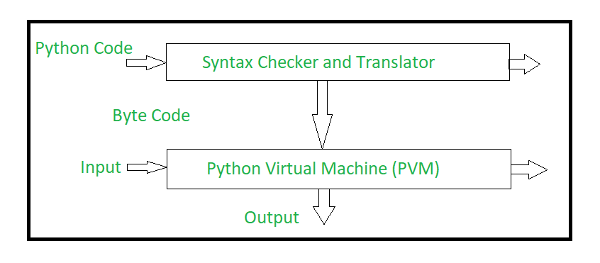
Internal working of Python
Python way of Data Science
Python provide great functionality to deal with mathematics, statistics and scientific function. It provides great libraries to deals with data science application.
- It’s Flexible
- It’s Easy to Learn
- It’s Open Source
- It’s Well-Supported
As is the case with many other programming languages, it’s the available libraries that lead to Python’s success: some 72,000 of them in the Python Package Index (PyPI) and growing constantly.
Python
# print the integers from 1 to 0
for i in range(1,10):
    print(i)
Java
// print the integers from 1 to 9
for(int i=1;i<10;i++){
  System.out.println(i);
}
Python hanldes a lot of memory automatically, so less time dealing with pointers and references and so on than other lanugages like C++.
Developer who prioritize ease of programming over execution speed
Python runs slower than other common languages like C++ or Java, but its often quick to write (three to five times faster than Java and five to ten times than C++).
One of the main reason why Python is used in "support language" for tasks like build control, automated testing and bug tracking. For the same reason used for prototyping.
Developers working with text and numbers
Python have powerful String anf List manipulation functions. Its a great tool for exploring data.
Avoiding the need for compiling makes it easier to run interactively on data for step by step manipulation. (Just like this Jupyter notebook).
Python's core functionality can be extended with a huge number of packages which are mainly used by the scientific and academic communities as well as engineering.
These include the Numpy(mathematical function and data analysis), SciPy(for science), Matplotlib(data visualization) and Pandas(data analysis) and more recently Tensorflow and Keras (Machine Learning/AI) and tens of thousands of others.
Web Developers
Backend development for webapplication. Python has built-in supports for common protocols like HTML, XML and Json.
Frameworks like Django, Flask and Bottle are widely used. For example Reddit's backend in Python.
The Zen of Python
The Zen of Python is a collection of 19 "guiding principles".
Some are:
- Readability counts.
- Simple is better than complex
- There should be one - and preferably only one - obvious way to do it.
Intro to Data Processing, Statistical analysis and Visualization libraries
A Brief Note on Python Versions
As of Janurary 1, 2020, Python has officially dropped support for python2.
!python --version
Python 3.7.11
Numpy is the core library for scientific computing in Python. It provides a high-performance multidimensional array object, and tools for working with these arrays.
To use Numpy, we first need to import the numpy package:
import numpy as np
Arrays
A numpy array is a grid of values, all of the same type, and is indexed by a tuple of nonnegative integers. The number of dimensions is the rank of the array; the shape of an array is a tuple of integers giving the size of the array along each dimension.
We can initialize numpy arrays from nested Python lists, and access elements using square brackets:
a = np.array([1, 2, 3])  # Create a rank 1 array
print(type(a), a.shape, a[0], a[1], a[2])
a[0] = 5                 # Change an element of the array
print(a)
<class 'numpy.ndarray'> (3,) 1 2 3
[5 2 3]
b = np.array([[1,2,3],[4,5,6]])   # Create a rank 2 array
print(b)
[[1 2 3]
 [4 5 6]]
print(b.shape)
print(b[0, 0], b[0, 1], b[1, 0])
(2, 3)
1 2 4
Numpy also provides many functions to create arrays:
a = np.zeros((2,2))  # Create an array of all zeros
print(a)
[[0. 0.]
 [0. 0.]]
b = np.ones((1,2))   # Create an array of all ones
print(b)
[[1. 1.]]
c = np.full((2,2), 7) # Create a constant array
print(c)
[[7 7]
 [7 7]]
d = np.eye(2)        # Create a 2x2 identity matrix
print(d)
[[1. 0.]
 [0. 1.]]
e = np.random.random((2,2)) # Create an array filled with random values
print(e)
[[0.18008187 0.07831069]
 [0.3829961  0.69663983]]
Array indexing
Numpy offers several ways to index into arrays.
Slicing: Similar to Python lists, numpy arrays can be sliced. Since arrays may be multidimensional, you must specify a slice for each dimension of the array:
import numpy as np

# Create the following rank 2 array with shape (3, 4)
# [[ 1  2  3  4]
#  [ 5  6  7  8]
#  [ 9 10 11 12]]
a = np.array([[1,2,3,4], [5,6,7,8], [9,10,11,12]])

# Use slicing to pull out the subarray consisting of the first 2 rows
# and columns 1 and 2; b is the following array of shape (2, 2):
# [[2 3]
#  [6 7]]
b = a[:2, 1:3]
print(b)
[[2 3]
 [6 7]]
A slice of an array is a view into the same data, so modifying it will modify the original array.
print(a[0, 1])
b[0, 0] = 77    # b[0, 0] is the same piece of data as a[0, 1]
print(a[0, 1])
2
77
You can also mix integer indexing with slice indexing. However, doing so will yield an array of lower rank than the original array.
# Create the following rank 2 array with shape (3, 4)
a = np.array([[1,2,3,4], [5,6,7,8], [9,10,11,12]])
print(a)
[[ 1  2  3  4]
 [ 5  6  7  8]
 [ 9 10 11 12]]
Two ways of accessing the data in the middle row of the array. Mixing integer indexing with slices yields an array of lower rank, while using only slices yields an array of the same rank as the original array:
row_r1 = a[1, :]    # Rank 1 view of the second row of a
row_r2 = a[1:2, :]  # Rank 2 view of the second row of a
row_r3 = a[[1], :]  # Rank 2 view of the second row of a
print(row_r1, row_r1.shape)
print(row_r2, row_r2.shape)
print(row_r3, row_r3.shape)
[5 6 7 8] (4,)
[[5 6 7 8]] (1, 4)
[[5 6 7 8]] (1, 4)
# We can make the same distinction when accessing columns of an array:
col_r1 = a[:, 1]
col_r2 = a[:, 1:2]
print(col_r1, col_r1.shape)
print()
print(col_r2, col_r2.shape)
[ 2  6 10] (3,)

[[ 2]
 [ 6]
 [10]] (3, 1)
Boolean array indexing: Boolean array indexing lets you pick out arbitrary elements of an array. Frequently this type of indexing is used to select the elements of an array that satisfy some condition. Here is an example:
import numpy as np

a = np.array([[1,2], [3, 4], [5, 6]])

bool_idx = (a > 2)  # Find the elements of a that are bigger than 2;
                    # this returns a numpy array of Booleans of the same
                    # shape as a, where each slot of bool_idx tells
                    # whether that element of a is > 2.

print(bool_idx)
[[False False]
 [ True  True]
 [ True  True]]
# We use boolean array indexing to construct a rank 1 array
# consisting of the elements of a corresponding to the True values
# of bool_idx
print(a[bool_idx])

# We can do all of the above in a single concise statement:
print(a[a > 2])
[3 4 5 6]
[3 4 5 6]
Datatypes
Every numpy array is a grid of elements of the same type. Numpy provides a large set of numeric datatypes that you can use to construct arrays. Numpy tries to guess a datatype when you create an array, but functions that construct arrays usually also include an optional argument to explicitly specify the datatype. Here is an example:
x = np.array([1, 2])  # Let numpy choose the datatype
y = np.array([1.0, 2.0])  # Let numpy choose the datatype
z = np.array([1, 2], dtype=np.int64)  # Force a particular datatype

print(x.dtype, y.dtype, z.dtype)
int64 float64 int64
You can read all about numpy datatypes in the documentation.
Array math
Basic mathematical functions operate elementwise on arrays, and are available both as operator overloads and as functions in the numpy module:
x = np.array([[1,2],[3,4]], dtype=np.float64)
y = np.array([[5,6],[7,8]], dtype=np.float64)

# Elementwise sum; both produce the array
print(x + y)
print(np.add(x, y))
[[ 6.  8.]
 [10. 12.]]
[[ 6.  8.]
 [10. 12.]]
# Elementwise difference; both produce the array
print(x - y)
print(np.subtract(x, y))
[[-4. -4.]
 [-4. -4.]]
[[-4. -4.]
 [-4. -4.]]
# Elementwise product; both produce the array
print(x * y)
print(np.multiply(x, y))
[[ 5. 12.]
 [21. 32.]]
[[ 5. 12.]
 [21. 32.]]
# Elementwise division; both produce the array
# [[ 0.2         0.33333333]
#  [ 0.42857143  0.5       ]]
print(x / y)
print(np.divide(x, y))
[[0.2        0.33333333]
 [0.42857143 0.5       ]]
[[0.2        0.33333333]
 [0.42857143 0.5       ]]
# Elementwise square root; produces the array
# [[ 1.          1.41421356]
#  [ 1.73205081  2.        ]]
print(np.sqrt(x))
[[1.         1.41421356]
 [1.73205081 2.        ]]
x = np.array([[1,2],[3,4]])
y = np.array([[5,6],[7,8]])

v = np.array([9,10])
w = np.array([11, 12])

# Inner product of vectors; both produce 219
print(v.dot(w))
print(np.dot(v, w))
219
219
You can also use the @ operator which is equivalent to numpy's dot operator.
print(v @ w)
219
# Matrix / vector product; both produce the rank 1 array [29 67]
print(x.dot(v))
print(np.dot(x, v))
print(x @ v)
[29 67]
[29 67]
[29 67]
# Matrix / matrix product; both produce the rank 2 array
# [[19 22]
#  [43 50]]
print(x.dot(y))
print(np.dot(x, y))
print(x @ y)
[[19 22]
 [43 50]]
[[19 22]
 [43 50]]
[[19 22]
 [43 50]]
Numpy provides many useful functions for performing computations on arrays; one of the most useful is sum:
x = np.array([[1,2],[3,4]])

print(np.sum(x))  # Compute sum of all elements; prints "10"
print(np.sum(x, axis=0))  # Compute sum of each column; prints "[4 6]"
print(np.sum(x, axis=1))  # Compute sum of each row; prints "[3 7]"
10
[4 6]
[3 7]
You can find the full list of mathematical functions provided by numpy in the documentation.
Apart from computing mathematical functions using arrays, we frequently need to reshape or otherwise manipulate data in arrays. The simplest example of this type of operation is transposing a matrix; to transpose a matrix, simply use the T attribute of an array object:
print(x)
print("transpose\n", x.T)
[[1 2]
 [3 4]]
transpose
 [[1 3]
 [2 4]]
v = np.array([[1,2,3]])
print(v )
print("transpose\n", v.T)
[[1 2 3]]
transpose
 [[1]
 [2]
 [3]]
pandas is a column-oriented data analysis API. It's a great tool for handling and analyzing input data, and many ML frameworks support pandas data structures as inputs. For a more complete reference, the pandas docs site contains extensive documentation and many tutorials.
Basic Concepts
The following line imports the pandas API and prints the API version:
from __future__ import print_function

import pandas as pd
pd.__version__
'1.1.5'
The primary data structures in pandas are implemented as two classes:
DataFrame, which you can imagine as a relational data table, with rows and named columns.Series, which is a single column. ADataFramecontains one or moreSeriesand a name for eachSeries.
The data frame is a commonly used abstraction for data manipulation. Similar implementations exist in Spark and R.
One way to create a Series is to construct a Series object. For example:
pd.Series(['San Francisco', 'San Jose', 'Sacramento'])
0    San Francisco
1         San Jose
2       Sacramento
dtype: object
DataFrame objects can be created by passing a dict mapping string column names to their respective Series. If the Series don't match in length, missing values are filled with special NA/NaN values. Example:
city_names = pd.Series(['San Francisco', 'San Jose', 'Sacramento'])
population = pd.Series([852469, 1015785, 485199])

pd.DataFrame({ 'City name': city_names, 'Population': population })
| City name | Population | |
|---|---|---|
| 0 | San Francisco | 852469 |
| 1 | San Jose | 1015785 |
| 2 | Sacramento | 485199 |
But most of the time, you load an entire file into a DataFrame. The following example loads a file with California housing data. Run the following cell to load the data and create feature definitions:
One way to create a Series is to construct a Series object. For example:
pd.Series(['San Francisco', 'San Jose', 'Sacramento'])
0    San Francisco
1         San Jose
2       Sacramento
dtype: object
DataFrame objects can be created by passing a dict mapping string column names to their respective Series. If the Series don't match in length, missing values are filled with special NA/NaN values. Example:
city_names = pd.Series(['San Francisco', 'San Jose', 'Sacramento'])
population = pd.Series([852469, 1015785, 485199])

pd.DataFrame({ 'City name': city_names, 'Population': population })
| City name | Population | |
|---|---|---|
| 0 | San Francisco | 852469 |
| 1 | San Jose | 1015785 |
| 2 | Sacramento | 485199 |
But most of the time, you load an entire file into a DataFrame. The following example loads a file with California housing data.
california_housing_dataframe = pd.read_csv("https://download.mlcc.google.com/mledu-datasets/california_housing_train.csv", sep=",")
california_housing_dataframe.describe()
| longitude | latitude | housing_median_age | total_rooms | total_bedrooms | population | households | median_income | median_house_value | |
|---|---|---|---|---|---|---|---|---|---|
| count | 17000.000000 | 17000.000000 | 17000.000000 | 17000.000000 | 17000.000000 | 17000.000000 | 17000.000000 | 17000.000000 | 17000.000000 |
| mean | -119.562108 | 35.625225 | 28.589353 | 2643.664412 | 539.410824 | 1429.573941 | 501.221941 | 3.883578 | 207300.912353 |
| std | 2.005166 | 2.137340 | 12.586937 | 2179.947071 | 421.499452 | 1147.852959 | 384.520841 | 1.908157 | 115983.764387 |
| min | -124.350000 | 32.540000 | 1.000000 | 2.000000 | 1.000000 | 3.000000 | 1.000000 | 0.499900 | 14999.000000 |
| 25% | -121.790000 | 33.930000 | 18.000000 | 1462.000000 | 297.000000 | 790.000000 | 282.000000 | 2.566375 | 119400.000000 |
| 50% | -118.490000 | 34.250000 | 29.000000 | 2127.000000 | 434.000000 | 1167.000000 | 409.000000 | 3.544600 | 180400.000000 |
| 75% | -118.000000 | 37.720000 | 37.000000 | 3151.250000 | 648.250000 | 1721.000000 | 605.250000 | 4.767000 | 265000.000000 |
| max | -114.310000 | 41.950000 | 52.000000 | 37937.000000 | 6445.000000 | 35682.000000 | 6082.000000 | 15.000100 | 500001.000000 |
The example above used DataFrame.describe to show interesting statistics about a DataFrame. Another useful function is DataFrame.head, which displays the first few records of a DataFrame:
california_housing_dataframe.head()
| longitude | latitude | housing_median_age | total_rooms | total_bedrooms | population | households | median_income | median_house_value | |
|---|---|---|---|---|---|---|---|---|---|
| 0 | -114.31 | 34.19 | 15.0 | 5612.0 | 1283.0 | 1015.0 | 472.0 | 1.4936 | 66900.0 |
| 1 | -114.47 | 34.40 | 19.0 | 7650.0 | 1901.0 | 1129.0 | 463.0 | 1.8200 | 80100.0 |
| 2 | -114.56 | 33.69 | 17.0 | 720.0 | 174.0 | 333.0 | 117.0 | 1.6509 | 85700.0 |
| 3 | -114.57 | 33.64 | 14.0 | 1501.0 | 337.0 | 515.0 | 226.0 | 3.1917 | 73400.0 |
| 4 | -114.57 | 33.57 | 20.0 | 1454.0 | 326.0 | 624.0 | 262.0 | 1.9250 | 65500.0 |
Another powerful feature of pandas is graphing. For example, DataFrame.hist lets you quickly study the distribution of values in a column:
california_housing_dataframe.hist('housing_median_age')
array([[<matplotlib.axes._subplots.AxesSubplot object at 0x7f559b178d50>]],
      dtype=object)

Accessing Data
You can access DataFrame data using familiar Python dict/list operations:
cities = pd.DataFrame({ 'City name': city_names, 'Population': population })
print(type(cities['City name']))
cities['City name']
<class 'pandas.core.series.Series'>
0    San Francisco
1         San Jose
2       Sacramento
Name: City name, dtype: object
print(type(cities['City name'][1]))
cities['City name'][1]
<class 'str'>
'San Jose'
print(type(cities[0:2]))
cities[0:2]
<class 'pandas.core.frame.DataFrame'>
| City name | Population | |
|---|---|---|
| 0 | San Francisco | 852469 |
| 1 | San Jose | 1015785 |
In addition, pandas provides an extremely rich API for advanced indexing and selection that is too extensive to be covered here.
Manipulating Data
You may apply Python's basic arithmetic operations to Series. For example:
population / 1000.
0     852.469
1    1015.785
2     485.199
dtype: float64
Modifying DataFrames is also straightforward. For example, the following code adds two Series to an existing DataFrame:
cities['Area square miles'] = pd.Series([46.87, 176.53, 97.92])
cities['Population density'] = cities['Population'] / cities['Area square miles']
cities
| City name | Population | Area square miles | Population density | |
|---|---|---|---|---|
| 0 | San Francisco | 852469 | 46.87 | 18187.945381 |
| 1 | San Jose | 1015785 | 176.53 | 5754.177760 |
| 2 | Sacramento | 485199 | 97.92 | 4955.055147 |
Indexes
Both Series and DataFrame objects also define an index property that assigns an identifier value to each Series item or DataFrame row.
By default, at construction, pandas assigns index values that reflect the ordering of the source data. Once created, the index values are stable; that is, they do not change when data is reordered.
city_names.index
RangeIndex(start=0, stop=3, step=1)
cities.index
RangeIndex(start=0, stop=3, step=1)
Call DataFrame.reindex to manually reorder the rows. For example, the following has the same effect as sorting by city name:
cities.reindex([2, 0, 1])
| City name | Population | Area square miles | Population density | |
|---|---|---|---|---|
| 2 | Sacramento | 485199 | 97.92 | 4955.055147 |
| 0 | San Francisco | 852469 | 46.87 | 18187.945381 |
| 1 | San Jose | 1015785 | 176.53 | 5754.177760 |
SciPy
%matplotlib inline
import matplotlib.pyplot as plt
from IPython.display import Image
The SciPy framework builds on top of the low-level NumPy framework for multidimensional arrays, and provides a large number of higher-level scientific algorithms. Some of the topics that SciPy covers are:
- Special functions (scipy.special)
- Integration (scipy.integrate)
- Optimization (scipy.optimize)
- Interpolation (scipy.interpolate)
- Fourier Transforms (scipy.fftpack)
- Signal Processing (scipy.signal)
- Linear Algebra (scipy.linalg)
- Sparse Eigenvalue Problems (scipy.sparse)
- Statistics (scipy.stats)
- Multi-dimensional image processing (scipy.ndimage)
- File IO (scipy.io)
Each of these submodules provides a number of functions and classes that can be used to solve problems in their respective topics.
To access the SciPy package in a Python program, we start by importing everything from the scipy module.
from scipy import *
If we only need to use part of the SciPy framework we can selectively include only those modules we are interested in. For example, to include the linear algebra package under the name la, we can do:
import scipy.linalg as la
Special functions
A large number of mathematical special functions are important for many computional physics problems. SciPy provides implementations of a very extensive set of special functions. For details, see the list of functions in the reference documention at http://docs.scipy.org/doc/scipy/reference/special.html#module-scipy.special.
To demonstrate the typical usage of special functions we will look in more detail at the Bessel functions:
Integration
Numerical integration: quadrature
Numerical evaluation of a function of the type
$\displaystyle \int_a^b f(x) dx$
is called numerical quadrature, or simply quadature. SciPy provides a series of functions for different kind of quadrature, for example the quad, dblquad and tplquad for single, double and triple integrals, respectively.
from scipy.integrate import quad, dblquad, tplquad
Ordinary differential equations (ODEs)
SciPy provides two different ways to solve ODEs: An API based on the function odeint, and object-oriented API based on the class ode. Usually odeint is easier to get started with, but the ode class offers some finer level of control.
Here we will use the odeint functions. For more information about the class ode, try help(ode). It does pretty much the same thing as odeint, but in an object-oriented fashion.
For example, to use odeint, import it from the scipy.integrate module
from scipy.integrate import odeint, ode
Fourier transform
Fourier transforms are one of the universal tools in computational physics, which appear over and over again in different contexts. SciPy provides functions for accessing the classic FFTPACK library from NetLib, which is an efficient and well tested FFT library written in FORTRAN. The SciPy API has a few additional convenience functions, but overall the API is closely related to the original FORTRAN library.
To use the fftpack module in a python program, include it using:
from numpy.fft import fftfreq
from scipy.fftpack import *
Linear algebra
The linear algebra module contains a lot of matrix related functions, including linear equation solving, eigenvalue solvers, matrix functions (for example matrix-exponentiation), a number of different decompositions (SVD, LU, cholesky), etc.
Detailed documetation is available at: http://docs.scipy.org/doc/scipy/reference/linalg.html
Optimization
Optimization (finding minima or maxima of a function) is a large field in mathematics, and optimization of complicated functions or in many variables can be rather involved. Here we will only look at a few very simple cases. For a more detailed introduction to optimization with SciPy see: http://scipy-lectures.github.com/advanced/mathematical_optimization/index.html
To use the optimization module in scipy first include the optimize module:
from scipy import optimize
Interpolation
Interpolation is simple and convenient in scipy: The interp1d function, when given arrays describing X and Y data, returns and object that behaves like a function that can be called for an arbitrary value of x (in the range covered by X), and it returns the corresponding interpolated y value:
Statistics
The scipy.stats module contains a large number of statistical distributions, statistical functions and tests. For a complete documentation of its features, see http://docs.scipy.org/doc/scipy/reference/stats.html.
There is also a very powerful python package for statistical modelling called statsmodels. See http://statsmodels.sourceforge.net for more details.
Matplotlib
Matplotlib is a plotting library. In this section give a brief introduction to the matplotlib.pyplot module, which provides a plotting system similar to that of MATLAB.
import matplotlib.pyplot as plt
By running this special iPython command, we will be displaying plots inline:
%matplotlib inline
Plotting
The most important function in matplotlib is plot, which allows you to plot 2D data. Here is a simple example:
# Compute the x and y coordinates for points on a sine curve
x = np.arange(0, 3 * np.pi, 0.1)
y = np.sin(x)

# Plot the points using matplotlib
plt.plot(x, y)
[<matplotlib.lines.Line2D at 0x7f558e85dd50>]

With just a little bit of extra work we can easily plot multiple lines at once, and add a title, legend, and axis labels:
y_sin = np.sin(x)
y_cos = np.cos(x)

# Plot the points using matplotlib
plt.plot(x, y_sin)
plt.plot(x, y_cos)
plt.xlabel('x axis label')
plt.ylabel('y axis label')
plt.title('Sine and Cosine')
plt.legend(['Sine', 'Cosine'])
<matplotlib.legend.Legend at 0x7f558e7e6950>

Subplots
You can plot different things in the same figure using the subplot function. Here is an example:
# Compute the x and y coordinates for points on sine and cosine curves
x = np.arange(0, 3 * np.pi, 0.1)
y_sin = np.sin(x)
y_cos = np.cos(x)

# Set up a subplot grid that has height 2 and width 1,
# and set the first such subplot as active.
plt.subplot(2, 1, 1)

# Make the first plot
plt.plot(x, y_sin)
plt.title('Sine')

# Set the second subplot as active, and make the second plot.
plt.subplot(2, 1, 2)
plt.plot(x, y_cos)
plt.title('Cosine')

# Show the figure.
plt.show()

You can read much more about the subplot function in the documentation.
Seaborn
Reference: Visualization-With-Seaborn
Seaborn. Seaborn provides an API on top of Matplotlib that offers sane choices for plot style and color defaults, defines simple high-level functions for common statistical plot types, and integrates with the functionality provided by Pandas DataFrames.
Seaborn Versus Matplotlib
Here is an example of a simple random-walk plot in Matplotlib, using its classic plot formatting and colors. We start with the typical imports:
import matplotlib.pyplot as plt
plt.style.use('classic')
%matplotlib inline
import numpy as np
import pandas as pd
Now we create some random walk data:
# Create some data
rng = np.random.RandomState(0)
x = np.linspace(0, 10, 500)
y = np.cumsum(rng.randn(500, 6), 0)
And do a simple plot:
# Plot the data with Matplotlib defaults
plt.plot(x, y)
plt.legend('ABCDEF', ncol=2, loc='upper left');

Although the result contains all the information we'd like it to convey, it does so in a way that is not all that aesthetically pleasing, and even looks a bit old-fashioned in the context of 21st-century data visualization.
Now let's take a look at how it works with Seaborn.
As we will see, Seaborn has many of its own high-level plotting routines, but it can also overwrite Matplotlib's default parameters and in turn get even simple Matplotlib scripts to produce vastly superior output.
We can set the style by calling Seaborn's set() method.
By convention, Seaborn is imported as sns:
import seaborn as sns
sns.set()
Now let's rerun the same two lines as before:
# same plotting code as above!
plt.plot(x, y)
plt.legend('ABCDEF', ncol=2, loc='upper left');

Exploring Seaborn Plots
The main idea of Seaborn is that it provides high-level commands to create a variety of plot types useful for statistical data exploration, and even some statistical model fitting.
Let's take a look at a few of the datasets and plot types available in Seaborn. Note that all of the following could be done using raw Matplotlib commands (this is, in fact, what Seaborn does under the hood) but the Seaborn API is much more convenient.
Histograms, KDE, and densities
Often in statistical data visualization, all you want is to plot histograms and joint distributions of variables. We have seen that this is relatively straightforward in Matplotlib:
data = np.random.multivariate_normal([0, 0], [[5, 2], [2, 2]], size=2000)
data = pd.DataFrame(data, columns=['x', 'y'])

for col in 'xy':
    plt.hist(data[col], normed=True, alpha=0.5)
---------------------------------------------------------------------------
AttributeError                            Traceback (most recent call last)
<ipython-input-64-7c25cafad82f> in <module>()
      3
      4 for col in 'xy':
----> 5     plt.hist(data[col], normed=True, alpha=0.5)

/usr/local/lib/python3.7/dist-packages/matplotlib/pyplot.py in hist(x, bins, range, density, weights, cumulative, bottom, histtype, align, orientation, rwidth, log, color, label, stacked, data, **kwargs)
   2608         align=align, orientation=orientation, rwidth=rwidth, log=log,
   2609         color=color, label=label, stacked=stacked, **({"data": data}
-> 2610         if data is not None else {}), **kwargs)
   2611
   2612

/usr/local/lib/python3.7/dist-packages/matplotlib/__init__.py in inner(ax, data, *args, **kwargs)
   1563     def inner(ax, *args, data=None, **kwargs):
   1564         if data is None:
-> 1565             return func(ax, *map(sanitize_sequence, args), **kwargs)
   1566
   1567         bound = new_sig.bind(ax, *args, **kwargs)

/usr/local/lib/python3.7/dist-packages/matplotlib/axes/_axes.py in hist(self, x, bins, range, density, weights, cumulative, bottom, histtype, align, orientation, rwidth, log, color, label, stacked, **kwargs)
   6817             if patch:
   6818                 p = patch[0]
-> 6819                 p.update(kwargs)
   6820                 if lbl is not None:
   6821                     p.set_label(lbl)

/usr/local/lib/python3.7/dist-packages/matplotlib/artist.py in update(self, props)
   1004
   1005         with cbook._setattr_cm(self, eventson=False):
-> 1006             ret = [_update_property(self, k, v) for k, v in props.items()]
   1007
   1008         if len(ret):

/usr/local/lib/python3.7/dist-packages/matplotlib/artist.py in <listcomp>(.0)
   1004
   1005         with cbook._setattr_cm(self, eventson=False):
-> 1006             ret = [_update_property(self, k, v) for k, v in props.items()]
   1007
   1008         if len(ret):

/usr/local/lib/python3.7/dist-packages/matplotlib/artist.py in _update_property(self, k, v)
   1000                 if not callable(func):
   1001                     raise AttributeError('{!r} object has no property {!r}'
-> 1002                                          .format(type(self).__name__, k))
   1003                 return func(v)
   1004

AttributeError: 'Rectangle' object has no property 'normed'

Rather than a histogram, we can get a smooth estimate of the distribution using a kernel density estimation, which Seaborn does with sns.kdeplot:
for col in 'xy':
    sns.kdeplot(data[col], shade=True)
Histograms and KDE can be combined using distplot:
sns.distplot(data['x'])
sns.distplot(data['y']);
If we pass the full two-dimensional dataset to kdeplot, we will get a two-dimensional visualization of the data:
sns.kdeplot(data);
We can see the joint distribution and the marginal distributions together using sns.jointplot.
For this plot, we'll set the style to a white background:
with sns.axes_style('white'):
    sns.jointplot("x", "y", data, kind='kde');
There are other parameters that can be passed to jointplot—for example, we can use a hexagonally based histogram instead:
with sns.axes_style('white'):
    sns.jointplot("x", "y", data, kind='hex')
Pair plots
When you generalize joint plots to datasets of larger dimensions, you end up with pair plots. This is very useful for exploring correlations between multidimensional data, when you'd like to plot all pairs of values against each other.
We'll demo this with the well-known Iris dataset, which lists measurements of petals and sepals of three iris species:
iris = sns.load_dataset("iris")
iris.head()
Visualizing the multidimensional relationships among the samples is as easy as calling sns.pairplot:
sns.pairplot(iris, hue='species', size=2.5);
Plotly
Plotly Python is an open-source library built on top of plotly.js which allows users to create professional quality, interactive, web-based or standalone visualizations or applications.
Visualizations can be displayed in Jupyter notebooks, standalone HTML files, or integrated into web-applications via the Dash framework.
Over 40 unique charts and limitless customization options exist across statistical, financial, geographic, scientific, and 3-D plot types. (from plotly website)
There are a couple more notes in regards to Plotly that is needed to be shared:
Plotly - Online
Plotly - Enterprise
Intro to Model Building and inference frameworks
scikit-learn
Reference: Scientific Python Stanford University
Scikit-learn is a library that allows you to do machine learning, that is, make predictions from data, in Python. There are four basic machine learning tasks:
- Regression: predict a number from datapoints, given datapoints and corresponding numbers
- Classification: predict a category from datapoints, given datapoints and corresponding numbers
- Clustering: predict a category from datapoints, given only datapoints
- Dimensionality reduction: make datapoints lower-dimensional so that we can visualize the data
Here is a handy flowchart of when to use each technique.

import pandas as pd
import numpy as np
import matplotlib.pyplot as plt
Regression
Abalone are a type of edible marine snail, and they have internal rings that correspond to their age (like trees). In the following, we will use a dataset of abalone measurements. It has the following fields:
Sex / nominal / -- / M, F, and I (infant)
Length / continuous / mm / Longest shell measurement
Diameter	/ continuous / mm / perpendicular to length
Height / continuous / mm / with meat in shell
Whole weight / continuous / grams / whole abalone
Shucked weight / continuous	/ grams / weight of meat
Viscera weight / continuous / grams / gut weight (after bleeding)
Shell weight / continuous / grams / after being dried
Rings / integer / -- / +1.5 gives the age in years
Suppose we are interested in predicting the age of the abalone given their measurements. This is an example of a regression problem.
df = pd.read_csv('http://archive.ics.uci.edu/ml/machine-learning-databases/abalone/abalone.data',
                   header=None, names=['sex', 'length', 'diameter', 'height', 'weight', 'shucked_weight',
                                       'viscera_weight', 'shell_weight', 'rings'])
df.head()
df.describe()
df['rings'].plot(kind='hist')
df.plot('weight', 'rings', kind='scatter')
X = df[['weight']].to_numpy()
y = df['rings'].to_numpy()
X
y
from sklearn import linear_model
model = linear_model.LinearRegression()
model.fit(X, y)
print(model.coef_, model.intercept_)
print(model.score(X, y))
model.predict(np.array([[1.5], [2.2]]))
df.plot('weight', 'rings', kind='scatter')

weight = np.linspace(0, 3, 10).reshape(-1, 1)
plt.plot(weight, model.predict(weight), 'r')
df['root_weight'] = np.sqrt(df['weight'])
X = df[['weight','root_weight']].to_numpy()
y = df['rings'].to_numpy()
model = linear_model.LinearRegression()
model.fit(X, y)
weight = np.linspace(0, 3, 100).reshape(-1, 1)
root_weight = np.sqrt(weight)

features = np.hstack((weight,root_weight))
df.plot('weight', 'rings', kind='scatter')

plt.plot(weight, model.predict(features), 'r')
model.score(X,y)
plt.hist2d(df['weight'],df['rings'],bins=(50,30));
Classification
Another example of a machine learning problem is classification. Here we will use a dataset of flower measurements from three different flower species of Iris (Iris setosa, Iris virginica, and Iris versicolor). We aim to predict the species of the flower. Because the species is not a numerical output, it is not a regression problem, but a classification problem.
from sklearn import datasets
iris = datasets.load_iris()
print(iris.DESCR)
X = iris.data[:, 2:]
y = iris.target_names[iris.target]
for name in iris.target_names:
    plt.scatter(X[y == name, 0], X[y == name, 1], label=name)
plt.xlabel('Petal length')
plt.ylabel('Petal width')
plt.legend();
from sklearn.model_selection import train_test_split
X_train, X_test, y_train, y_test = train_test_split(X, y, test_size=0.2, random_state=0)
print(X_train.shape, y_train.shape)
print(X_test.shape, y_test.shape)
from sklearn.neighbors import KNeighborsClassifier
model = KNeighborsClassifier()
model.fit(X_train, y_train)
X_test
model.predict(X_test)
import sklearn.metrics as metrics
metrics.accuracy_score(model.predict(X_test), y_test)
print(metrics.classification_report(model.predict(X_test), y_test))
Clustering
Clustering is useful if we don't have a dataset labelled with the categories we want to predict, but we nevertheless expect there to be a certain number of categories. For example, suppose we have the previous dataset, but we are missing the labels. We can use a clustering algorithm like k-means to cluster the datapoints. Because we don't have labels, clustering is what is called an unsupervised learning algorithm.
from sklearn.datasets import make_blobs
X,y = make_blobs(centers=4, n_samples=200, random_state=0, cluster_std=0.7)
print(X[:10],y[:10])
Now we plot these points, but without coloring the points using the labels:
plt.scatter(X[:,0],X[:,1]);
We can still discern four clusters in the data set. Let's see if the k-means algorithm can recover these clusters. First we create the instance of the k-means model by giving it the number of clusters 4 as a hyperparameter.
from sklearn.cluster import KMeans
model = KMeans(4)
model.fit(X)
print(model.cluster_centers_)
plt.scatter(X[:,0],X[:,1], c=model.labels_);
plt.scatter(model.cluster_centers_[:,0], model.cluster_centers_[:,1], s=100, color="red"); # Show the centres
Dimensionality reduction
Dimensionality reduction is another unsupervised learning problem (that is, it does not require labels). It aims to project datapoints into a lower dimensional space while preserving distances between datapoints.
 Tensorflow
TensorFlow is an end-to-end open source platform for machine learning.
TensorFlow was originally created by Google as an internal machine learning tool, but an implementation of it was open sourced under the Apache 2.0 License in November 2015.
Few reason for the popluarity of tensorflow
- Python API
- Portability: deploy computation to one or more CPUs or GPUs in a esktop, server, or mobile device with a single API
- Flexibility: from Raspberry Pi, Android, Windows, iOS, Linux to server farms
- Visualization
- Checkpoints (for managing experiments)
- Large community (> 10,000 commits and > 3000 TF-related repos in one year)
- Awesome projects already using TensorFlow
Reference: Tensorflow beginner
import tensorflow as tf
Load and prepare the MNIST dataset. Convert the samples from integers to floating-point numbers:
mnist = tf.keras.datasets.mnist

(x_train, y_train), (x_test, y_test) = mnist.load_data()
x_train, x_test = x_train / 255.0, x_test / 255.0
Build the tf.keras.Sequential model by stacking layers. Choose an optimizer and loss function for training:
model = tf.keras.models.Sequential([
  tf.keras.layers.Flatten(input_shape=(28, 28)),
  tf.keras.layers.Dense(128, activation='relu'),
  tf.keras.layers.Dropout(0.2),
  tf.keras.layers.Dense(10)
])
model.compile(optimizer='adam',
              loss='sparse_categorical_crossentropy',
              metrics=['accuracy'])
The Model.fit method adjusts the model parameters to minimize the loss:
model.fit(x_train, y_train, epochs=5)
The Model.evaluate method checks the models performance, usually on a "Validation-set" or "Test-set".
model.evaluate(x_test, y_test, verbose=2)
The image classifier is now trained to ~98% accuracy on this dataset. To learn more, read the TensorFlow tutorials.
Pytorch
PyTorch is a machine learning framework that is used in both academia and industry for various applications. An alternative to tensorflow
---
3. Approaching a Tabular Problem
Titanic Survivor Prediction Challenge

3.1 Understanding the Problem
This challenge is kind of a "hello world" program in the whole data Science and Machine Learning community.
The task is simple,use machine learning to create a model that predicts which passengers survived the Titanic shipwreck. In this challenge, we perform a basic EDA and build a predictive model that answers the question: “what sorts of people were more likely to survive?” using passenger data (ie name, age, gender, socio-economic class, etc).
While there was some element of luck involved in surviving, it seems some groups of people were more likely to survive than others.
Contents
1. Data Description
2. Exploratory Data Analysis
3. Findings From EDA
4. Data Preprocessing
5. Feature Engineering and Feature Selection
6. Data Modeling and Evaluation
* Logistic Regression
* Gradient Boosting Classifier
* XgBoost
* SGB Classifier
7. Models Comparison
Data Description
- Survival : 0 = No, 1 = Yes
- pclass(Ticket Class) : 1 = 1st, 2 = 2nd, 3 = 3rd
- Sex(Gender) : Male, Female
- Age : Age in years
- SibSp : Number of siblings/spouses abroad the titanic
- Parch : Number of parents/children abrod the titanic
- Ticket : Ticket Number
- Fare : Passenger fare
- Cabin : Cabin Number
- Embarked : Port of Embarkation, C = Cherbourg, Q = Queenstown, S = Southampton
import pandas as pd
import numpy as np
import matplotlib.pyplot as plt
import seaborn as sns

import warnings
warnings.filterwarnings('ignore')

plt.style.use('fivethirtyeight')
%matplotlib inline
#loading a CSV file using pandas dataframe
train_df = pd.read_csv('./inputs/tab/train.csv')
train_df.head()
#Fetching some statistical information of the data
train_df.describe()
#Information about a DataFrame including the index dtype and columns, non-null values and memory usage
train_df.info()
# Checking for null values
train_df.isna().sum()
Exploratory Data Analysis (EDA)
Exploratory Data Analysis refers to the critical process of performing initial investigations on data so as to discover patterns,to spot anomalies,to test hypothesis and to check assumptions with the help of summary statistics and graphical representations
# visualizing null values
import missingno as msno

msno.bar(train_df)
plt.show()
# Correlation and mulitcolinarity
plt.figure(figsize = (18, 8))
corr = train_df.corr()

sns.heatmap(corr, annot = True, fmt = '.2f', linewidths = 1, annot_kws = {'size' : 15})
plt.show()
Survived Column - Target
plt.figure(figsize = (12, 7))

sns.countplot(y = 'Survived', data = train_df)
plt.show()
#pie chart to show Survived vs Not in percentage
values = train_df['Survived'].value_counts()
labels = ['Not Survived', 'Survived']

fig, ax = plt.subplots(figsize = (5, 5), dpi = 100)
explode = (0, 0.06)

patches, texts, autotexts = ax.pie(values, labels = labels, autopct = '%1.2f%%', shadow = True,
                                   startangle = 90, explode = explode)

plt.setp(texts, color = 'grey')
plt.setp(autotexts, size = 12, color = 'white')
autotexts[1].set_color('black')
plt.show()
Pclass Column
#individual count of each class
train_df.Pclass.value_counts()
#Individual counts of Pclass based on Target
train_df.groupby(['Pclass', 'Survived'])['Survived'].count()
#bar chart showing Pclass counts based on Targets
plt.figure(figsize = (16, 8))

sns.countplot('Pclass', hue = 'Survived', data = train_df)
plt.show()
#Pie chart showing Pclass counts percentage based on Targets
values = train_df['Pclass'].value_counts()
labels = ['Third Class', 'Second Class', 'First Class']
explode = (0, 0, 0.08)
fig, ax = plt.subplots(figsize = (5, 6), dpi = 100)
patches, texts, autotexts = ax.pie(values, labels = labels, autopct = '%1.2f%%', shadow = True,
                                   startangle = 90, explode = explode)
plt.setp(texts, color = 'grey')
plt.setp(autotexts, size = 13, color = 'white')
autotexts[2].set_color('black')
plt.show()
Name Column
#Count of uniqes names
train_df.Name.value_counts()
len(train_df.Name.unique()), train_df.shape
Gender Column
#Count of Male vs Female grouped on Target
train_df.groupby(['Sex', 'Survived'])['Survived'].count()
#Individual counts of Gender based on Target
plt.figure(figsize = (16, 7))

sns.countplot('Sex', hue = 'Survived', data = train_df)
plt.show()
#Individual counts of Gender based on Target for each Pclass Category
sns.catplot(x = 'Sex', y = 'Survived', data = train_df, kind = 'bar', col = 'Pclass')
plt.show()
Age Column
#Age distribution
plt.figure(figsize = (15, 6))
plt.style.use('ggplot')

sns.distplot(train_df['Age'])
plt.show()
#Checking outliers in Age grouped by Gender
sns.catplot(x = 'Sex', y = 'Age', kind = 'box', data = train_df, height = 5, aspect = 2)
plt.show()
#Checking outliers in Age grouped by Gender and Pclass
sns.catplot(x = 'Sex', y = 'Age', kind = 'box', data = train_df, col = 'Pclass')
plt.show()
Cabin Column

Fare Column
#Histogram showing Fare counts
plt.figure(figsize = (14, 6))

plt.hist(train_df.Fare, bins = 60, color = 'orange')
plt.xlabel('Fare')
plt.show()
#outliers in Fare based on Gender and Pclass
sns.catplot(x = 'Sex', y = 'Fare', data = train_df, kind = 'box', col = 'Pclass')
plt.show()
SibSp Column
#Count of people with Siblings or spouse
train_df['SibSp'].value_counts()
#count of people with Sibilings or Spouse based on Target
plt.figure(figsize = (16, 5))

sns.countplot(x = 'SibSp', data = train_df, hue = 'Survived')
plt.show()
#Count of people who survived based on SibSp counts
sns.catplot(x = 'SibSp', y = 'Survived', kind = 'bar', data = train_df, height = 5, aspect =2)
plt.show()
#Count of people who survived based on SibSp counts Gender wise
sns.catplot(x = 'SibSp', y = 'Survived', kind = 'bar', hue = 'Sex', data = train_df, height = 6, aspect = 2)
plt.show()
sns.catplot(x = 'SibSp',  y = 'Survived', kind = 'bar', col = 'Sex', data = train_df)
plt.show()
#Count of people who survived based on SibSp counts Gender and Pclass wise
sns.catplot(x = 'SibSp', y = 'Survived', col = 'Pclass', kind = 'bar', data = train_df)
plt.show()
Parch Column
#Count of people with Parents/Childrens
train_df.Parch.value_counts()
sns.catplot(x = 'Parch', y = 'Survived', data = train_df, hue = 'Sex', kind = 'bar', height = 6, aspect = 2)
plt.show()
Ticket Column
#count based on ticket types
train_df.Ticket.value_counts()
len(train_df.Ticket.unique())
Embarked Column
train_df['Embarked'].value_counts()
#Count of people based on Port Embarked Gender wise
plt.figure(figsize = (14, 6))

sns.countplot('Embarked', hue = 'Survived', data = train_df)
plt.show()
sns.catplot(x = 'Embarked', y = 'Survived', kind = 'bar', data = train_df, col = 'Sex')
plt.show()
Findings From EDA :-
- Females Survived more than Males.
- Passengers Travelling in Higher Class Survived More than Passengers travelling in Lower Class.
- Name column is having all unique values so this column is not suitable for prediction, we have to drop it.
- In First Class Females were more than Males, that's why Fare of Females Passengers were high.
- Survival Rate is higher for those who were travelling with siblings or spouses.
- Passengers travelling with parents or children have higher survival rate.
- Ticket column is not useful and does not have an impact on survival.
- Cabin column have a lot of null values , it will be better to drop this column.
- Passengers travelling from Cherbourg port survived more than passengers travelling from other two ports.
3.2 Data Preprocessing
# dropping useless columns with noise, missing data ..etc
train_df.drop(['PassengerId', 'Name', 'Ticket', 'Cabin'], axis = 1, inplace = True)
train_df.head()
train_df.isna().sum()
# replacing Zero values of "Fare" column with mean of column
train_df['Fare'] = train_df['Fare'].replace(0, train_df['Fare'].mean())
# filling null values of "Age" column with mean value of the column

train_df['Age'].fillna(train_df['Age'].mean(), inplace = True)
# filling null values of "Embarked" column with mode value of the column

train_df['Embarked'].fillna(train_df['Embarked'].mode()[0], inplace = True)
# checking for null values after filling null values

train_df.isna().sum()
train_df.head()
3.4 Feature Engineering and Feature Selection
'''
Not all Machine Leanrning Algorithms like categorical fearures as strings,
so they need to me encoded to numeric formats so they these alorithms can ingest this data without throwing error
labelEncoding : Converting String to numeric format'''
train_df['Sex'] = train_df['Sex'].apply(lambda val: 1 if val == 'male' else 0)
train_df.head()
OneHot Encoding : It is the representation of categorical variables as binary vectors

# Get one hot encoding of columns 'Embarked'
one_hot = pd.get_dummies(train_df['Embarked'])
# Drop column 'Embarked' as it is now encoded
train_df = train_df.drop('Embarked',axis = 1)
# Join the encoded train_df
train_df = train_df.join(one_hot)
train_df.head()
train_df.describe()
#checking for feature variance is very important
#High variance can affect the model performance, espcially for Linear models
#so we need to normalize high variance features
train_df.var()
#log normalization
train_df['Age'] = np.log(train_df['Age'])
train_df['Fare'] = np.log(train_df['Fare'])
test_df = pd.read_csv('./inputs/tab/test.csv')
test_df.head()
# dropping useless columns
test_df.drop(['PassengerId', 'Name', 'Ticket', 'Cabin'], axis = 1, inplace = True)
# replacing Zero values of "Fare" column with mean of column
test_df['Fare'] = test_df['Fare'].replace(0, test_df['Fare'].mean())
# filling null values of "Age" column with mean value of the column
test_df['Age'].fillna(test_df['Age'].mean(), inplace = True)
# filling null values of "Embarked" column with mode value of the column
test_df['Embarked'].fillna(test_df['Embarked'].mode()[0], inplace = True)
test_df.isna().sum()
# filling null values of "Fare" column with mean value of the column
test_df['Fare'].fillna(test_df['Fare'].mean(), inplace = True)
test_df['Sex'] = test_df['Sex'].apply(lambda val: 1 if val == 'male' else 0)

# Get one hot encoding of columns 'Embarked'
one_hot_test = pd.get_dummies(test_df['Embarked'])
# Drop column 'Embarked' as it is now encoded
test_df = test_df.drop('Embarked',axis = 1)
# Join the encoded train_df
test_df = test_df.join(one_hot_test)
# Log Normalization
test_df['Age'] = np.log(test_df['Age'])
test_df['Fare'] = np.log(test_df['Fare'])
test_df.head()
test_df.var()
test_df.isna().any()
test_df.head()
# Dividing data to features and targets
X = train_df.drop('Survived', axis = 1)
y = train_df['Survived']
# splitting data intp training and test set

from sklearn.model_selection import train_test_split

X_train, X_test, y_train, y_test = train_test_split(X, y, test_size = 0.30, random_state = 0)
Data Modeling
Training Machine Learning models to predict survivors
1. Logistic Regression
from sklearn.linear_model import LogisticRegression

lr = LogisticRegression()
lr.fit(X_train, y_train)

# accuracy score, confusion matrix and classification report of logistic regression

from sklearn.metrics import accuracy_score, confusion_matrix, classification_report

lr_acc = accuracy_score(y_test, lr.predict(X_test))

print(f"Training Accuracy of Logistic Regression is {accuracy_score(y_train, lr.predict(X_train))}")
print(f"Test Accuracy of Logistic Regression is {lr_acc}")

print(f"Confusion Matrix :- \n {confusion_matrix(y_test, lr.predict(X_test))}")
print(f"Classofocation Report : -\n {classification_report(y_test, lr.predict(X_test))}")
# hyper parameter tuning of logistic regression
from sklearn.model_selection import GridSearchCV

grid_param = {
    'penalty': ['l1', 'l2'],
    'C' : [0.001, 0.01, 0.1, 0.005, 0.5, 1, 10]
}

grid_search_lr = GridSearchCV(lr, grid_param, cv = 5, n_jobs = -1, verbose = 1)
grid_search_lr.fit(X_train, y_train)
# best parameters and best score

print(grid_search_lr.best_params_)
print(grid_search_lr.best_score_)
# best estimator

lr = grid_search_lr.best_estimator_

# accuracy score, confusion matrix and classification report of logistic regression

lr_acc = accuracy_score(y_test, lr.predict(X_test))

print(f"Training Accuracy of Logistic Regression is {accuracy_score(y_train, lr.predict(X_train))}")
print(f"Test Accuracy of Logistic Regression is {lr_acc}")

print(f"Confusion Matrix :- \n {confusion_matrix(y_test, lr.predict(X_test))}")
print(f"Classofocation Report : -\n {classification_report(y_test, lr.predict(X_test))}")
2. Random Forest
from sklearn.ensemble import RandomForestClassifier

rd_clf = RandomForestClassifier()
rd_clf.fit(X_train, y_train)

# accuracy score, confusion matrix and classification report of random forest

rd_clf_acc = accuracy_score(y_test, rd_clf.predict(X_test))

print(f"Training Accuracy of Decision Tree Classifier is {accuracy_score(y_train, rd_clf.predict(X_train))}")
print(f"Test Accuracy of Decision Tree Classifier is {rd_clf_acc} \n")

print(f"Confusion Matrix :- \n{confusion_matrix(y_test, rd_clf.predict(X_test))}\n")
print(f"Classification Report :- \n {classification_report(y_test, rd_clf.predict(X_test))}")
3. Gradient Boosting
from sklearn.ensemble import GradientBoostingClassifier

gb = GradientBoostingClassifier()
gb.fit(X_train, y_train)

# accuracy score, confusion matrix and classification report of gradient boosting classifier

gb_acc = accuracy_score(y_test, gb.predict(X_test))

print(f"Training Accuracy of Decision Tree Classifier is {accuracy_score(y_train, gb.predict(X_train))}")
print(f"Test Accuracy of Decision Tree Classifier is {gb_acc} \n")

print(f"Confusion Matrix :- \n{confusion_matrix(y_test, gb.predict(X_test))}\n")
print(f"Classification Report :- \n {classification_report(y_test, gb.predict(X_test))}")
4. Stochastic Gradient Boosting (SGB)
sgb = GradientBoostingClassifier(subsample = 0.90, max_features = 0.70)
sgb.fit(X_train, y_train)

# accuracy score, confusion matrix and classification report of stochastic gradient boosting classifier

sgb_acc = accuracy_score(y_test, sgb.predict(X_test))

print(f"Training Accuracy of Decision Tree Classifier is {accuracy_score(y_train, sgb.predict(X_train))}")
print(f"Test Accuracy of Decision Tree Classifier is {sgb_acc} \n")

print(f"Confusion Matrix :- \n{confusion_matrix(y_test, sgb.predict(X_test))}\n")
print(f"Classification Report :- \n {classification_report(y_test, sgb.predict(X_test))}")
5. XGboost
from xgboost import XGBClassifier

xgb = XGBClassifier(booster = 'gbtree', learning_rate = 0.1, max_depth = 5, n_estimators = 180)
xgb.fit(X_train, y_train)

# accuracy score, confusion matrix and classification report of xgboost

xgb_acc = accuracy_score(y_test, xgb.predict(X_test))

print(f"Training Accuracy of Decision Tree Classifier is {accuracy_score(y_train, xgb.predict(X_train))}")
print(f"Test Accuracy of Decision Tree Classifier is {xgb_acc} \n")

print(f"Confusion Matrix :- \n{confusion_matrix(y_test, xgb.predict(X_test))}\n")
print(f"Classification Report :- \n {classification_report(y_test, xgb.predict(X_test))}")
Model Comparison
models = pd.DataFrame({
    'Model' : ['Logistic Regression', 'Gradient Boosting Classifier', 'Stochastic Gradient Boosting', 'XgBoost'],
    'Score' : [lr_acc,gb_acc, sgb_acc, xgb_acc]
})

models.sort_values(by = 'Score', ascending = False)
plt.figure(figsize = (15, 10))

sns.barplot(x = 'Score', y = 'Model', data = models)
plt.show()
Real Data Model Inference
pred_class = {0: 'Not Survived', 1: 'Survived'}
def predict(test_input, test_target):
    final_results = gb.predict([test_input])
    test_input['Age'] = np.exp(test_input['Age'])
    test_input['Fare'] = np.exp(test_input['Fare'])
    print(f"Features:\n{test_input}\n\nClassifier prediction: {pred_class[final_results.item()]}\nActual Target: {pred_class[test_target]}")
test_input = X.iloc[0,:]
test_target = y.iloc[0]
predict(test_input, test_target)
test_input = X.iloc[1,:]
test_target = y.iloc[1]
predict(test_input, test_target)
4. Approaching a Text (NLP) Problem

4.1 Importance of solving NLP
NLP — also known as computational linguistics — is the combination of AI and linguistics that allows us to talk to machines as if they were human.
In other words, NLP is an approach to process, analyze and understand large amount of text data.

1. Handling large volumes of text data
With the big data technology, NLP has entered the mainstream as this approach can now be applied to handle large volumes of text data via cloud/distributed computing at an unprecedented speed.
2. Structuring highly unstructured data source
Human language is astoundingly complex and diverse.
NLP is important because it helps resolve ambiguity in language and adds useful numeric structure to the data for many downstream applications, such as speech recognition or text analytics.
Components of NLP
NLP can be divided into two basic components.
- Natural Language Understanding
- Natural Language Generation
Natural Language Understanding (NLU)
There are lot of ambiguity while learning or trying to interpret a language.
- Lexical Ambiguity can occur when a word carries different sense
- Syntactical Ambiguity means when we see more than one meaning in a sequence of words.
- Referential Ambiguity: Very often a text mentions as entity (something/someone),
Natural Language Generation (NLG)
It involves :
- Text planning − It includes retrieving the relevant content from knowledge base.
- Sentence planning − It includes choosing required words, forming meaningful phrases, setting tone of the sentence.
- Text Realization − It is mapping sentence plan into sentence structure.
Applications of NLP
Search Autocorrect and Autocomplete

Language Translator

Chatbots

Sentiment analysis

4.3 Basics of NLP
Corpus
A corpus is a large and structured set of machine-readable texts that have been produced in a natural communicative setting. Its plural is corpora. They can be derived in different ways like text that was originally electronic, transcripts of spoken language and optical character recognition, etc.
Tokens
The raw text is a sequence of characters (bytes), but most times it is useful to group those characters into contiguous units called tokens. In English, tokens correspond to words and numeric sequences separated by white-space characters or punctuation.
Tokenization
The process of breaking a text down into tokens is called tokenization.It can become more complicated than simply splitting text based on nonalphanumeric characters.
N-grams
They are basically a set of co-occurring words within a given window and when computing the n-grams you typically move one word forward. Trigram has three token, bigram has two tokens, a unigram one.
Stemming
Stemming algorithms work by cutting off the end or the beginning of the word, taking into account a list of common prefixes and suffixes that can be found in an inflected word.Stemming just removes the last few characters, often leading to incorrect meanings and spelling errors
Lemmatization
Lemmatization is similar to stemming but it brings context to the words. So it links words with similar meaning to one word.
4.4 NLP using Python
NLTK
It is a leading platform for building Python programs to work with human language data. It provides easy-to-use interfaces to over 50 corpora and lexical resources such as WordNet, along with a suite of text processing libraries for classification, tokenization, stemming, tagging, parsing, and semantic reasoning, wrappers for industrial-strength NLP libraries
spaCy
It is an open-source software library for advanced natural language processing, written in the programming languages Python and Cython.Unlike NLTK, which is widely used for teaching and research, spaCy focuses on providing software for production usage.spaCy also supports deep learning workflows that allow connecting statistical models trained by popular machine learning libraries like TensorFlow, PyTorch or MXNet through its own machine learning library Thinc
4.5 Approaching real life NLP problem
Intro to Twitter tweets processing using Python

Problem Statement
With all of the tweets circulating every second it is hard to tell whether the sentiment behind a specific tweet will impact a company, or a person's, brand for being viral (positive), or devastate profit because it strikes a negative tone. Capturing sentiment in language is important in these times where decisions and reactions are created and updated in seconds. In order to get the sentiments out of tweets they need to by processed to tweaked in ways so that it could be fed into a algorithm to perform to sentiment inference. So we will take a look at pythonic approach of processing tweets
import pandas as pd
import matplotlib.pyplot as plt
import seaborn as sns
import numpy as np
from nltk.corpus import stopwords
from nltk.util import ngrams
from sklearn.feature_extraction.text import CountVectorizer
from sklearn.feature_extraction.text import TfidfVectorizer
from wordcloud import WordCloud, STOPWORDS
from nltk.stem.wordnet import WordNetLemmatizer
from nltk import word_tokenize
from collections import defaultdict
from collections import  Counter
plt.style.use('ggplot')
stop=set(stopwords.words('english'))
import re
from nltk.tokenize import word_tokenize
import gensim
import string
from tqdm import tqdm
tweet=pd.read_csv("./inputs/nlp/train.csv")
test=pd.read_csv("./inputs/nlp/test.csv")
tweet.head(100)
print('There are {} rows and {} columns in train'.format(tweet.shape[0],tweet.shape[1]))
print('There are {} rows and {} columns in train'.format(test.shape[0],test.shape[1]))
Class Distribution
Before we begin with anything else,let's check the class distribution.There are only two classes 0 and 1.
x=tweet.target.value_counts()
sns.barplot(x.index,x)
plt.gca().set_ylabel('samples')
Exploratory Data Analysis (EDA)
#First,we will do very basic analysis,that is character level,word level and sentence level analysis.
fig,(ax1,ax2)=plt.subplots(1,2,figsize=(10,5))
tweet_len=tweet[tweet['target']==1]['text'].str.len()
ax1.hist(tweet_len,color='red')
ax1.set_title('disaster tweets')
tweet_len=tweet[tweet['target']==0]['text'].str.len()
ax2.hist(tweet_len,color='green')
ax2.set_title('Not disaster tweets')
fig.suptitle('Characters in tweets')
plt.show()

print("The distribution of both seems to be almost same.120 t0 140 characters in a tweet are the most common among both.")
# Number of words in tweet
fig,(ax1,ax2)=plt.subplots(1,2,figsize=(10,5))
tweet_len=tweet[tweet['target']==1]['text'].str.split().map(lambda x: len(x))
ax1.hist(tweet_len,color='red')
ax1.set_title('disaster tweets')
tweet_len=tweet[tweet['target']==0]['text'].str.split().map(lambda x: len(x))
ax2.hist(tweet_len,color='green')
ax2.set_title('Not disaster tweets')
fig.suptitle('Words in a tweet')
plt.show()

print("Most of disaster tweets are around between 10 -20 word counts\nand Non disaster tweet areound 15 to 20")
# Average word length in a tweet
fig,(ax1,ax2)=plt.subplots(1,2,figsize=(10,5))
word=tweet[tweet['target']==1]['text'].str.split().apply(lambda x : [len(i) for i in x])
sns.distplot(word.map(lambda x: np.mean(x)),ax=ax1,color='red')
ax1.set_title('disaster')
word=tweet[tweet['target']==0]['text'].str.split().apply(lambda x : [len(i) for i in x])
sns.distplot(word.map(lambda x: np.mean(x)),ax=ax2,color='green')
ax2.set_title('Not disaster')
fig.suptitle('Average word length in each tweet')
Creating Corpus
We need to perform further EDA we need corpus
#creating text corpus based on target
#corpus of Disaster vs Non Disaster Tweet

def build_corpus(target):
    corpus=[]

    for x in tweet[tweet['target']==target]['text'].str.split():
        for i in x:
            corpus.append(i)
    return corpus
#wordcloud of non disaster tweets
comment_words = ''
stopwords = set(STOPWORDS)
comment_words += " ".join(build_corpus(0))+" "

wordcloud = WordCloud(width = 800, height = 800,
                background_color ='white',
                stopwords = stopwords,
                min_font_size = 10).generate(comment_words)

plt.figure(figsize = (8, 8), facecolor = None)
plt.imshow(wordcloud)
plt.axis("off")
plt.tight_layout(pad = 0)
plt.show()
#wordcloud of disaster tweets
comment_words = ''
stopwords = set(STOPWORDS)
comment_words += " ".join(build_corpus(1))+" "

wordcloud = WordCloud(width = 800, height = 800,
                background_color ='black',
                stopwords = stopwords,
                min_font_size = 10).generate(comment_words)

plt.figure(figsize = (8, 8), facecolor = None)
plt.imshow(wordcloud)
plt.axis("off")
plt.tight_layout(pad = 0)

plt.show()
#creating corpus based of Non Disaster Tweet
corpus=build_corpus(0)

#build dicr based on NoN disaster tweet
dic=defaultdict(int)
for word in corpus:
    if word in stop:
        dic[word]+=1

#choosing top tweets
top=sorted(dic.items(), key=lambda x:x[1],reverse=True)[:10]
top
#bar chart showing common words in NoN disaster tweets
x,y = zip(*top)
plt.figure(figsize=(15,8))
plt.bar(x, y);
#creating the same for Diaster Tweet
corpus=build_corpus(1)

dic=defaultdict(int)
for word in corpus:
    if word in stop:
        dic[word]+=1

top=sorted(dic.items(), key=lambda x:x[1],reverse=True)[:10]

plt.figure(figsize=(15,8))
x,y=zip(*top)
plt.bar(x,y)
plt.show()

print("Words like 'the','in','of' dominates, but these words have not much meaning or prediction capabilities")
#Analysing punctuations for Disaster Tweets
plt.figure(figsize=(15,8))
corpus=build_corpus(1)

dic=defaultdict(int)
import string
special = string.punctuation
for i in (corpus):
    if i in special:
        dic[i]+=1

x,y=zip(*dic.items())
plt.title("Analysing punctuations for Disaster Tweets")
plt.bar(x,y,color='orange');
#Analysing punctuations for Non-Disaster Tweets
plt.figure(figsize=(15,8))
corpus=build_corpus(0)

dic=defaultdict(int)
import string
special = string.punctuation
for i in (corpus):
    if i in special:
        dic[i]+=1

x,y=zip(*dic.items())
plt.title("Analysing punctuations for Non-Disaster Tweets")
plt.bar(x,y,color='red');
#performing the same for complete corpus
complete_corpus = []
complete_corpus.extend(build_corpus(0))
complete_corpus.extend(build_corpus(1))
counter=Counter(corpus)
most=counter.most_common()
x=[]
y=[]
for word,count in most[:40]:
    if (word not in stop) :
        x.append(word)
        y.append(count)
plt.figure(figsize=(15,8))
sns.barplot(x=y,y=x).set_title("Complete corpus common words")
plt.show()
N-gram Analysis
We can perform Bigram and Trigram analysis on this data to understand word combinations in the dataset
def get_top_tweet_bigrams(corpus, gram=2, n=None):
    vec = CountVectorizer(ngram_range=(gram, gram)).fit(corpus)
    bag_of_words = vec.transform(corpus)
    sum_words = bag_of_words.sum(axis=0)
    words_freq = [(word, sum_words[0, idx]) for word, idx in vec.vocabulary_.items()]
    words_freq =sorted(words_freq, key = lambda x: x[1], reverse=True)
    return words_freq[:n]
#count of common bigrams
plt.figure(figsize=(15,8))
top_tweet_bigrams=get_top_tweet_bigrams(tweet['text'], gram=2)[:10]
x,y=map(list,zip(*top_tweet_bigrams))
sns.barplot(x=y,y=x).set_title("Common Bigram Count")
plt.show()
#count of common trigrams
plt.figure(figsize=(15,8))
top_tweet_trigrams=get_top_tweet_bigrams(tweet['text'], gram=3)[:10]
x,y=map(list,zip(*top_tweet_trigrams))
sns.barplot(x=y,y=x).set_title("Common Trigram Count")
plt.show()
After performing Bigram and Trigram analysis on this data clearly shows the need of data cleaning
Data Cleaning
Raw twitter data contains a lot of noise like stopwords, irrelavant punctuations, emojis ..etc which could kill its prediction capabilities. So let's clean them
df=pd.concat([tweet,test])
df.shape
Lemmatization
def lemma(text):
    text = text.lower()
    lmtzr = WordNetLemmatizer()
    text = " ".join([lmtzr.lemmatize(word) for word in word_tokenize(text)])
    return text

ex = "Our Deeds are the Reason of this #earthquake"
lemma(ex)
#apply lemmatization
df['text']=df['text'].apply(lambda x : lemma(x))
Removing URL
#Regex to remove URL
def remove_URL(text):
    url = re.compile(r'https?://\S+|www\.\S+')
    return url.sub(r'',text)

sample_URL = "please find the titanic project at https://www.kaggle.com/c/titanic/overview"
remove_URL(sample_URL)
#Apply the cleaning process
df['text']=df['text'].apply(lambda x : remove_URL(x))
df[['text','target']].head()
Removing HTML
#remove html
def remove_html(text):
    html=re.compile(r'<.*?>')
    return html.sub(r'',text)

sample_HTML = '''
<html>
<div>
<h1>Welcome to HTML</h>
<a href="https://www.kaggle.com/c/titanic/overview">kaggle</a>
<p>test paragraph</p>
</div>
</html>
'''
print(remove_html(sample_HTML))
df['text']=df['text'].apply(lambda x : remove_html(x))
df[['text','target']].head()
Removing Emojis 😔
Emoji's have great prediction capabilities but they need to be encoded to some numeric problem, Lets just remove it for simplicity sake
def remove_emoji(text):
    emoji_pattern = re.compile("["
                           u"\U0001F600-\U0001F64F"  # emoticons
                           u"\U0001F300-\U0001F5FF"  # symbols & pictographs
                           u"\U0001F680-\U0001F6FF"  # transport & map symbols
                           u"\U0001F1E0-\U0001F1FF"  # flags (iOS)
                           u"\U00002702-\U000027B0"
                           u"\U000024C2-\U0001F251"
                           "]+", flags=re.UNICODE)
    return emoji_pattern.sub(r'', text)
remove_emoji("its flooding i am scared 😔😔")
df['text']=df['text'].apply(lambda x: remove_emoji(x))
df[['text','target']].head()
Removing punctuations
Just like emojis punctuation also posses some kind of meaning like :) :( ..etc , But its hard to encode such punctation to numeric formats when vectorizing text. So we can remove it
def remove_punct(text):
    table=str.maketrans('','',string.punctuation)
    return text.translate(table)

example="There are #earthquakes"
print(remove_punct(example))
df['text']=df['text'].apply(lambda x : remove_punct(x))
df[['text','target']].head()
Vectorization
Text needs to be encoded to numerical format before we feed it into a machine learning algorithm
Bag-Of-Words - The model is simple in that it throws away all of the order information in the words and focuses on the occurrence of words in a document.

BOW vectorization techniques
1. convert text to word count vectors with CountVectorizer
2. convert text to word frequency vectors with TfidfVectorizer.
Word Counts with CountVectorizer
The CountVectorizer provides a simple way to both tokenize a collection of text documents and build a vocabulary of known words, but also to encode new documents using that vocabulary.
# list of text documents
text = ["heard about the earthquake is different city stay safe everyone and hope the city fast recovery"]
# create the transform
vectorizer = CountVectorizer()
# tokenize and build vocab
vectorizer.fit(text)
# summarize
print(vectorizer.vocabulary_)
# encode document
vector = vectorizer.transform(text)
# summarize encoded vector
print(vector.shape)
print(type(vector))
print(vector.toarray())
#vectorizing the whole tweet
vectorizer = CountVectorizer()
vectorizer.fit(df.text.values)
vector = vectorizer.transform(df.text.values)
print(vector.shape)
#to see the vocab dictionary
# print(vectorizer.vocabulary_)
Word Frequencies with TfidfVectorizer
TF-IDF are word frequency scores that try to highlight words that are more interesting, e.g. frequent in a document but not across documents.
* Term Frequency: This summarizes how often a given word appears within a document.
* Inverse Document Frequency: This downscales words that appear a lot across documents.
# list of text documents
text = ["The quick brown fox jumped over the lazy dog.","The dog.","The fox"]
# create the transform
vectorizer = TfidfVectorizer()
# tokenize and build vocab
vectorizer.fit(text)
# summarize
print(vectorizer.vocabulary_)
print(vectorizer.idf_)
# encode document
vector = vectorizer.transform([text[0]])
# summarize encoded vector
print(vector.shape)
print(vector.toarray())
vectorizer = TfidfVectorizer()
# tokenize and build vocab
vectorizer.fit(df.text.values);
# print(vectorizer.vocabulary_)
print(vectorizer.idf_.shape)
print(vectorizer.idf_)
vector = vectorizer.transform([text[0]])
# summarize encoded vector
print(vector.shape)
print(vector.toarray())
What is Computer Vision
Two definitions of computer vision:
Computer vision can be defined as
a scientific field that extracts information out of digital images. The type of
information gained from an image can vary from identification, space
measurements for navigation, or augmented reality applications.
Another way to define computer vision is through its applications.
Computer vision is building algorithms that can understand the content of images and use it for other applications.

Computer vision at the intersection of multiple scientific fields
Source: Computer Vision: Foundation and Applications by Ranjay Krishna - Stanford University

Source: Lecture'1: Introductionto Computer Vision by Prof. FeiBFei Li Stanford Vision Lab

Source: Lecture'1: Introductionto Computer Vision by Prof. FeiBFei Li Stanford Vision Lab
Why Computer Vision Matter

How is computer vision used today?
Optical character recognition (OCR)
Technology to convert scanned docs to text

License plate readers
Face detection

Face analysis and recognition

Login without a password

Special effects: shape capture

Special effects: motion capture

3D face tracking with consumer cameras

Image synthesis

Smart Cars

Self Driving Cars

Image synthesis
Challenges


Image Processing
Point Operators
The simplest kind of image processing transforms are point operators, where each output pixel value depends on only the corresponding input pixel value (plus some globally collected information or parameters)
Pixel Transforms
Pixel transforms are applying a funtion over each pixel value in the images. It can be a linear function with a gain and bias, which are used in brightness and contrast control, or can be a non-linear function which are used in gamma corrections in digital cameras
Color transforms
Brightening a picture by adding a constant value to all three color channels created undesired side effects like affecting its hue and saturation.
chromaticity coordinates or even simpler color ratios can first be computed and then used after manipulating (e.g., brightening) the luminance Y to re-compute a valid RGB image with the same hue and saturation.
Compositing and matting
The process of extracting the object from the original image is often called matting.
The process of inserting it into another image (without visible artifacts) is called compositing.

(a) Original Image (b) alpha-matted color image (c) alpha channel (d) Composited image
Histogram equalization
How can be determine the best values for brightness and gain controls?
The answer is to plot the histogram of the individual color channels and luminance values. From this distribution, we can compute relevant statistics such as the minimum, maximum, and average intensity values
Example: Histogram equalization


Linear Filtering
Neighborhood operator or local operator, which uses a collection of pixel values in the vicinity of a given pixel to determine its final output value.
In addition to performing local tone adjustment, neighborhood operators can be used to filter images to add soft blur, sharpen details, accentuate edges, or remove noise.
1. Seperable Filtering
The process of performing convolution operation can be sped up by a convolution kernel which is called seperable.
2. Band-pass and steerable filters
Band-pass filters filter out both low and high frequencies which kernel can be created by first smoothing the image with a Guassian filter and then taking the first or second derivatives.
More neighborhood operators
1. Non-linear filtering
Consider an image with 'shot noise', noise with occasioanlly large pixel values. Using a linear filter such as regular blurring with gaussian filter will only turn those large values into softer spots.
Median filtering
Selects the median value from each pixel’s neighborhood. Since the shot
noise value usually lies well outside the true values in the neighborhood, the median filter is able to filter away such bad pixels.
2. Bilateral filtering
In the bilateral filter, the output pixel value depends on a weighted combination of neighboring pixel values. The idea is to simply reject (in a soft way) pixels whose values differ too much from the central pixel value.
Binary image processing
Binary images are thresholded grey scale image with pixel value either 0 or 1.
Morphology
we first convolve the binary image with a binary structuring element and then select a binary output value depending on the thresholded result of the convolution.
Examples are dilation, erosion, majority, opening, closing
Distance Transforms
Also known as distance map or distance field, is a derived representation of a digital image.
The map labels each pixel of the image with the distance to the nearest obstacle pixel. A most common type of obstacle pixel is a boundary pixel in a binary image.
Fourier Transforms
Is used to decompose an image into its sine and cosine components. The output of the transformation represents the image in the Fourier or frequency domain, while the input image is the spatial domain equivalent.
The Fast Fourier Transforms is used to perform large-kernel operation in time that is independent of the kernel size.
Two-dimensional Fourier transforms
**Wiener filtering***
The fourier tranform can be sued to analyze the frequency spectrum of a whole class of image.
This linear filtering technique assumes that if noise is present in the system, then it is considered to be additive white Gaussian noise (AWGN). (*Not used in practice today)
Discrete cosine transform
The discrete cosine transform (DCT) is a variant of the Fourier transform particularly well suited to compressing images in a block-wise fashion.
The DCT is widely used in today’s image and video compression algorithms.
Pyramids and wavelets
We may need to alter the resolution of an image for speeding up an processing alogorithm or to match the resolution of a printer or a screen.
Interpolation
Image interpolation (or upsample) occurs when you resize or distort your image from one pixel grid to another.
Works by using known data to estimate values at unknown points. Common methods can be grouped into two categories:
Adaptive methods
Adaptive methods change depending on what they are interpolating. Examples include many proprietary algorithms in licensed software such as: Qimage, PhotoZoom Pro and Genuine Fractals.
Non-adaptive methods
Non-adaptive methods treat all pixels equally and examples are nearest neighbor, bilinear, bicubic, spline, sinc, lanczos etc.
A camera performs an optical zoom by moving the zoom lens so that it increases the magnification of light. However, a digital zoom degrades quality by simply interpolating the image. Even though the photo with digital zoom contains the same number of pixels, the detail is clearly far less than with optical zoom.
Decimation
Reducing resolution of an image (downsampling). This is done by convolving the image with a low-pass filter and then keep every rth sample. Some examples of decimations filters are Direct subsampling, Block averaging, Sinc function.
Applications include Image compression, Limited bandwidth image transmission etc.
Multi-resolution representations
Consider a task of finding a face in an image, since we don't know what is the size of the face in an image, we can construct a pyramid of differently sized images and scan each one for possible faces.
Laplacian pyramid
To construct the pyramid, we first blur and subsample the original image by a factor of two and store this in the next level of the pyramid. Also known as an octave pyramid.
Image pyramids are extremely useful for performing multi-scale editing operations such as blending images while maintaining details.
Wavelets
Wavelets provide a smooth way to decompose a signal into frequency components without blocking and are closely related to pyramids.
Continuous Wavelet Transform, Inverse continuous wavelet transform, Discrete Wavelet Transform are three main methods of wavelets transforms.
Application of wavelets include De-noising, Compression and Image fusion.
Geometric transformations
Parametric transformations
Parametric transformations apply a global deformation to an image, where the behavior of the transformation is controlled by a small number of parameters.
MIP-mapping
A MIP-map is a standard image pyramid, where each level is prefiltered with a high-quality filter rather than a poorer quality approximation.
Computer graphics rendering APIs, such as OpenGL and Direct3D, have parameters that can be used to select which variant of MIP-mapping should be used, depending on the desired tradeoff between speed and quality.
Anisotropic filtering
An alternative approach to filtering oriented textures, which is sometimes implemented in graphics hardware (GPUs), is to use anisotropic filtering.
Multi-pass transforms
The advantage of using a series of one-dimensional transforms is that they are much more efficient (in terms of basic arithmetic operations) than large, non-separable, two-dimensional filter kernels.
Mesh-based warping
For example, changing the appearance of a face from a frown to a smile, what is needed in this case is to curve the corners of the mouth upwards while leaving the rest of the face intact. To perform such a transformation, different amounts of motion are required in different parts of the image.
The mesh-warping algorithm relates features with nonuniform mesh in the source and destination images, i.e., the images are broken up into small regions that are mapped onto each other for the morph.
OpenCV
An opensource library which is supported by multiple platforms including Linux, Windows, Android and MacOS.
It supports a wide variety of programming languages such as C++, Python, Java etc.
OpenCV-Python is the Python API for OpenCV, combining the best qualities of the OpenCV C++ API and the Python language.
Pre-requisites
- Python 3.x
- Pip
To make sure that the Python version you currently have in your system is 3.x, run the below command on your systems terminal or command Prompt
$ python3 --version
To make sure that PIP package manager is installed on your system
$ pip3 --version
Or you can confirm the same by executing the below cells
! echo 'Python Version: '$(python3 --version)
! echo 'PIP Version: ' $(pip3 --version)
Installing OpenCV-Python
The OpenCV-Python package can be installed using the PIP package manager.
To install, run the below command on your terminal or command prompt
$ pip3 install opencv-python
You can do the same on this notebook as well, by executing the below cell
! pip3 install opencv-python
After installation is done, confirm the same by checking the version of the package
import cv2
print(f'OpenCV-Python Version: {cv2.__version__}')
Now, let's dive into OpenCV
Before diving into OpenCV, let's import few packages that we will be using throghout this notebook
- OpenCV
- Numpy
- Matplotlib
- os
run the below cell to import them
import os
import cv2 # OpenCV
import numpy as np
import matplotlib.pyplot as plt
%matplotlib inline
Let's set the path of the image directory
image_directory = 'images/'
Let's create a method to plot the images
# Method to plot the images
def plot_images(original, result=None):
"""Plot the images using matplotlib libray"""
# Plot single image
if result is None:
plt.imshow(cv2.cvtColor(original, cv2.COLOR_BGR2RGB))
plt.show()
return
#Plot two images
f, (axis1, axis2) = plt.subplots(1, 2, figsize=(15,15))
axis1.imshow(cv2.cvtColor(original, cv2.COLOR_BGR2RGB))
axis1.set_title('Origianl Image')
axis2.imshow(cv2.cvtColor(result, cv2.COLOR_BGR2RGB))
axis2.set_title('Resultant Image')
return
1. Changing colorspaces
There are more than 150 color-space conversion methods available in OpenCV. We will take a look at two of the widely used methods -
BGR ↔ Gray and BGR ↔ HSV
BGR - Blue-Green-Red
HSV - Hue- Saturation-Lightness
For color conversion, we can make use of the function cv.cvtColor(input_image, flag) where flag determines the type of conversion.
Here, we will try to extract a blue colored object from an image by following the below steps
- Read the image
- Convert from BGR to HSV color-space
- Threshold the HSV image for a range of blue color
# Read the input image
image = cv2.imread('images/color_spaces.jpg', cv2.IMREAD_COLOR)
# Plot the image using matplotlib
plot_images(image)
# Convert BGR to HSV
hsv = cv2.cvtColor(image, cv2.COLOR_BGR2HSV)
# define range of blue color in HSV
lower_blue = np.array([110,50,50])
upper_blue = np.array([130,255,255])
# Threshold the HSV image to get only blue colors
mask = cv2.inRange(hsv, lower_blue, upper_blue)
# Bitwise-AND mask and original image
res = cv2.bitwise_and(image, image, mask=mask)
# Plot the result image using matplotlib
plot_images(image, res)
2. Geometric Transformations of Images
1. Scaling
Scaling is just resizing of the image. OpenCV comes with a function cv.resize() for this purpose.
Preferable interpolation methods are
cv.INTER_AREAfor shrinkingcv.INTER_CUBIC(slow)cv.INTER_LINEARfor zooming
By default cv.INTER_LINEAR is used for all resizing purposes
Let's try resizing an image;
# Read the image
image = cv2.imread('images/color_spaces.jpg', cv2.IMREAD_COLOR)
# Plot the image using matplotlib
plot_images(image)
# Apply resize with `INTER_CUBIC` Interpolation - 10 times the size of input image
res = cv2.resize(image, None, fx=10, fy=10, interpolation = cv2.INTER_CUBIC)
print(f'Original size: {image.shape} \nResized image size: {res.shape}')
plot_images(res)
2. Translation
Translation is the shifting of an image along the x- and y-axis. Using translation, we can shift an image up, down, left, or right, along with any combination of the above.
If you want to rotate an image tx pixels along x-axis and ty pixels along y-axis, the tranformation matrix will be
[1, 0, tx][0, 1, ty]
Translation can be done by applying this transformation metrics to the method cv2.warpAffine().
# Read the image
image = cv2.imread('images/color_spaces.jpg', cv2.IMREAD_COLOR)
# Plot the image using matplotlib
plot_images(image)
# Shift the image 125 pixels to the right and 150 pixels down
M = np.float32([[1, 0, 125], [0, 1, 150]])
shifted = cv2.warpAffine(image, M, (image.shape[1], image.shape[0]))
# plot the image
plot_images(image, shifted)
# Shift the image 150 pixels to the left and 190 pixels up
M = np.float32([[1, 0, -150], [0, 1, -190]])
shifted = cv2.warpAffine(image, M, (image.shape[1], image.shape[0]))
# plot the image
plot_images(image, shifted)
3. Rotation
OpenCV provides a function, cv.getRotationMatrix2D to create a transformation matrix, which can be applied to the image using the method cv.warpAffine()
# Read the image
image = cv2.imread('images/color_spaces.jpg', cv2.IMREAD_COLOR)
# Plot the image using matplotlib
plot_images(image)
# grab the dimensions of the image and calculate the center of the image
(height, width) = image.shape[:2]
(cX, cY) = (width // 2, height // 2)
# rotate our image by 45 degrees around the center of the image
M = cv2.getRotationMatrix2D((cX, cY), 45, 1.0)
rotated = cv2.warpAffine(image, M, (width, height))
plot_images(image, rotated)
# rotate our image by -90 degrees around the image
M = cv2.getRotationMatrix2D((cX, cY), -90, 1.0)
rotated = cv2.warpAffine(image, M, (width, height))
plot_images(image, rotated)
5. Affine Transformation
To be added
6. Perspective Transformation
To be added
3. Image Thresholding
1. Simple Thresholding
For every pixel, a threshold value is applied. If the pixel value is smaller than the threshold, it is set to 0, otherwise it is set to a maximum value.
The function cv.threshold is used to apply the thresholding.
OpenCV provides different types of thresholding
cv.THRESH_BINARYcv.THRESH_BINARY_INVcv.THRESH_TRUNCcv.THRESH_TOZEROcv.THRESH_TOZERO_INV
Detailed explanation about this different methods can be found here.
Note: The input image must be a gray scale image
# read the input image
image = cv2.imread('images/simple_threshold.PNG',0)
# Plot the images
plot_images(image)
# Apply various thershold methods
ret,thresh1 = cv2.threshold(image,127,255,cv2.THRESH_BINARY)
ret,thresh2 = cv2.threshold(image,127,255,cv2.THRESH_BINARY_INV)
ret,thresh3 = cv2.threshold(image,127,255,cv2.THRESH_TRUNC)
ret,thresh4 = cv2.threshold(image,127,255,cv2.THRESH_TOZERO)
ret,thresh5 = cv2.threshold(image,127,255,cv2.THRESH_TOZERO_INV)
titles = ['Original Image','BINARY','BINARY_INV','TRUNC','TOZERO','TOZERO_INV']
images = [image, thresh1, thresh2, thresh3, thresh4, thresh5]
for i in range(6):
plt.subplot(2,3,i+1),plt.imshow(images[i],'gray',vmin=0,vmax=255)
plt.title(titles[i])
plt.xticks([]),plt.yticks([])
plt.show()
2. Adaptive Thresholding
Using one global value for thresholding might not be good in all cases eg. if the image has different lighting conditions in different areas.
Adaptive Thresholding determines the threshold for a pixel based on a small region around it. This can produce different thresholds for different regions of the same image which gives better results for image with varying illuminations. The method cv.adaptiveThreshold is used for it.
Two different methods of calculating the threshold
cv.ADAPTIVE_THRESH_MEAN_C: The threshold value is the mean of the neighbourhood area minus the constant C.cv.ADAPTIVE_THRESH_GAUSSIAN_C: The threshold value is a gaussian-weighted sum of the neighbourhood values minus the constant C.
The blockSize determines the size of the neighbourhood area and C is a constant that is subtracted from the mean or weighted sum of the neighbourhood pixels.
# Read the image
image = cv2.imread(f'{image_directory}calender.jpg',0)
# plot the image
plot_images(image)
# Apply the thresholding methods to the image
ret,thresh1 = cv2.threshold(image,127,255,cv2.THRESH_BINARY)
thresh2 = cv2.adaptiveThreshold(image,255,cv2.ADAPTIVE_THRESH_MEAN_C,\
cv2.THRESH_BINARY,11,2)
thresh3 = cv2.adaptiveThreshold(image,255,cv2.ADAPTIVE_THRESH_GAUSSIAN_C,\
cv2.THRESH_BINARY,11,2)
# Plot the thresholding resultant images
titles = ['Original Image', 'Global Thresholding (v = 127)',
'Adaptive Mean Thresholding', 'Adaptive Gaussian Thresholding']
plot_images(image, thresh1)
images = [image, thresh1, thresh2, thresh3]
for i in range(4):
plt.subplot(2,2,i+1),plt.imshow(images[i],'gray')
plt.title(titles[i])
plt.xticks([]),plt.yticks([])
plt.show()
3. Otsu's Binarization
Otsu's method avoids having to choose an arbitrary value as threshold and determines it automatically.
Determines an optimal global threshold value from the image histogram.
The cv.threshold() function is used, where cv.THRESH_OTSU is passed as an extra flag.
# Read input image
image = cv2.imread(f'{image_directory}periodic_table.png',0)
# Otsu's thresholding
ret2,thresh = cv2.threshold(image,0,255,cv2.THRESH_BINARY+cv2.THRESH_OTSU)
plot_images(image, thresh)
4. Smoothing Images
1. 2D Convolution ( Image Filtering )
As in one-dimensional signals, images also can be filtered with various low-pass filters (LPF), high-pass filters (HPF), etc. LPF helps in removing noise, blurring images, etc. HPF filters help in finding edges in images.
The function cv.filter2D() is used to convolve a kernel with an image.
For example, lets try applying the 5x5 averaging filter kernel below
kernel = np.ones((5,5),np.float32)/25
print(kernel)
The operation works like this: keep this kernel above a pixel, add all the 25 pixels below this kernel, take the average, and replace the central pixel with the new average value
# Read input image
image = cv2.imread(f'{image_directory}python_logo.png')
# Plot the image
plot_images(image)
# Apply the kernel
result = cv2.filter2D(image,-1,kernel)
plot_images(image, result)
2. Image Blurring (Image Smoothing)
Image blurring is achieved by convolving the image with a low-pass filter kernel. It is useful for removing noise.
OpenCV provides four different type of blurring techniques
1. Averaging
This is done by convolving an image with a normalized box filter. (as explained above in 2D convolution section)
The function cv.blur() can be used for averaging.
# apply the averaging kernel
blur = cv2.blur(image,(5,5))
# plot the image
plot_images(image, blur)
2. Gaussian Blurring
In this method, instead of a box filter, a Gaussian kernel is used. The function cv.GaussianBlur() is used.
Gaussian blurring is highly effective in removing Gaussian noise from an image.
# Apply gaussian blur
blur = cv2.GaussianBlur(image,(5,5),0)
# Plot the image
plot_images(image, blur)
3. Median Blurring
The function cv.medianBlur() takes the median of all the pixels under the kernel area and the central element is replaced with this median value.
Effective against removing salt and pepper noises.
# Add the Gaussian noise to the image - salt and pepper noise
# Generate Gaussian noise
gauss = np.random.normal(0,1,image.size)
gauss = gauss.reshape(image.shape[0],image.shape[1],image.shape[2]).astype('uint8')
# add generated noise to the image
image_gauss = cv2.add(image,gauss)
# Apply kernel to the image
median = cv2.medianBlur(image_gauss,5)
#plot the image
plot_images(image_gauss, median)
4. Bilateral Filtering
cv.bilateralFilter() is highly effective in noise removal while keeping edges sharp.
This filter preserve edges by considering Gaussian function of intensity difference that makes sure that only those pixels with similar intensities to the central pixel are considered for blurring.
# Load the input image
image = cv2.imread(f'{image_directory}pattern.PNG')
#plot the images
plot_images(image)
# Apply the filer
blur = cv2.bilateralFilter(image,25,75,75)
#plot the images
plot_images(image, blur)
5. Morphological Transformations
Morpholofical operations are simple operatins(kernels) performed on a binary image based on its shape.
# read the input image
image = cv2.imread(f'{image_directory}morphology.PNG')
# Plot the image
plot_images(image)
# create a 5x5 kernel
kernel = np.ones((5,5),np.uint8)
1. Erosion
Erodes the bounderies of a forground object.
Operaion of the erosion is as follows, a kernel slides through the image and if the pixel under the kernel is not 1, then its eroded(zero). Basically erodes the bounderies of an object.
It is useful for removing small white noises, detach two connected object etc.
# Apply the kenel to the input image
erosion = cv2.erode(image,kernel,iterations = 1)
# Plot the result image
plot_images(image, erosion)
2. Dilation
Dilation is opposite of erosion. A pixel element is 1, if atleast one pixel value under a kernel is 1.
# apply the kernel
dilation = cv2.dilate(image, kernel,iterations = 1)
# Plot the images
plot_images(image, dilation)
3. Opening
Opening is just another name of erosion followed by dilation.
Method used cv.morphologyEx()
Userful for removing whitenoise.
# Add the Gaussian noise to the image - salt and pepper noise
# Generate Gaussian noise
gauss = np.random.normal(0,0.5,image.size)
gauss = gauss.reshape(image.shape[0],image.shape[1],image.shape[2]).astype('uint8')
# add generated noise to the image
image_gauss = cv2.add(image,gauss)
# Apply the kernel
opening = cv2.morphologyEx(image_gauss, cv2.MORPH_OPEN, kernel)
# plot the image
plot_images(image_gauss, opening)
4. Closing
Closing is reverse of Opening, Dilation followed by Erosion.
It is useful in closing small holes inside the foreground objects, or small black points on the object.
# read the input image
image = cv2.imread(f'{image_directory}morphology_closing.PNG')
# apply the kernel
closing = cv2.morphologyEx(image, cv2.MORPH_CLOSE, kernel)
# Plot the images
plot_images(image, closing)
5. Morphological Gradient
It is the difference between dilation and erosion of an image.
# read the image
image = cv2.imread(f'{image_directory}morphology.PNG')
# Apply the kernel to the image
gradient = cv2.morphologyEx(image, cv2.MORPH_GRADIENT, kernel)
# Plot the images
plot_images(image, gradient)
6. Canny Edge Detection
Canny Edge Detection is a popular edge detection algorithm. It is a multistage alogorithm,
- Noise Reduction with a 5x5 Gaussian filter
- Finding Intensity Gradient of the Image
- Non-maximum Suppression to remove pixels which may not constitute the edges
- Hysteresis Thresholding to discard found edges based a threshold.
cv2.Canny() method is used for canny edge detection
# Read the input image
image = cv2.imread(f'{image_directory}stop_sign.jpg')
# Apply the canny edge detection
edges = cv2.Canny(image,50,200)
# Plot the images
plot_images(image, edges)
7. Image Pyramids
In case of working with images where we need to create a set of the same image with different resoultion, we can use Image Pyramids. At each layer of the pyramid the image is downsized or smoothed.
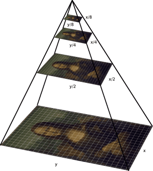
There are two types of image pyramids
- Gaussian Pyramid
- Laplacian Pyramids
We can find Gaussian pyramids using cv.pyrDown() and cv.pyrUp() functions.
Laplacian Pyramids are formed from the Gaussian Pyramids.
# Read input image
image = cv2.imread(f'{image_directory}stop_sign.jpg')
layer = image.copy()
# Plot the pyramid
for i in range(4):
layer = cv2.pyrDown(layer)
plot_images(layer)
8. Contours
Contours are simply as a curve joining all the continuous points (along the boundary), having same color or intensity. Useful tool for shape analysis and object detection and recognition.
OpenCV provides methods cv.findContours(), cv.drawContours() for the same.
In OpenCV, finding contours is like finding white object from black background.
# Read the image
image = cv2.imread(f'{image_directory}stop_sign.jpg')
org_image = image.copy()
# Convert the image from color to gray
imgray = cv2.cvtColor(image, cv2.COLOR_BGR2GRAY)
# Applying threshold
ret, thresh = cv2.threshold(imgray, 127, 255, 0)
# Find contours on the image
contours, hierarchy = cv2.findContours(thresh, cv2.RETR_TREE, cv2.CHAIN_APPROX_SIMPLE)
# Draw all the contours
contour_img = cv2.drawContours(image, contours, -1, (0,255,0), 3)
# Plot the image
plot_images(org_image, contour_img)
9. Histogram
You can consider histogram as a graph or plot, which gives you an overall idea about the intensity distribution of an image. It is a plot with pixel values (ranging from 0 to 255, not always) in X-axis and corresponding number of pixels in the image on Y-axis.

cv.calcHist() is used for calculing the histogram for a image.
Here, let us use the matplotlib library method to calculate the plot the histogram
# Read the input image
img = cv2.imread(f'{image_directory}stop_sign.jpg',0)
# plot the image
plot_images(img)
# Calculate histogram and plot
plt.hist(img.ravel(),256,[0,256]); plt.show()