Have you ever captured amazing underwater footage, only to discover that your photos were plagued by poor visibility, muted colours, and a bluish-green haze? You’re not by yourself. As depth increases, warmer colours such as red, orange, and yellow are absorbed first, leaving images looking dull and low in contrast. In this post, we are going to explore how these challenges can be addressed computationally using OpenCV, to restore colour balance, enhance contrast, and improve overall image clarity using simple yet effective image processing techniques in Python.
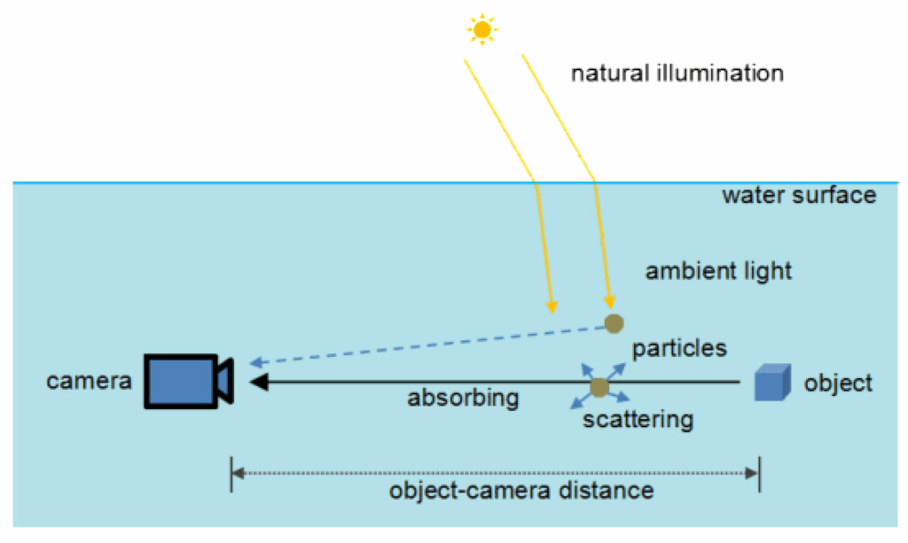
Table of contents
1. The Challenge: What Makes Underwater Images So Difficult?
Before diving into solutions, let us understand the enemy. Underwater images suffer from three primary degradation factors:
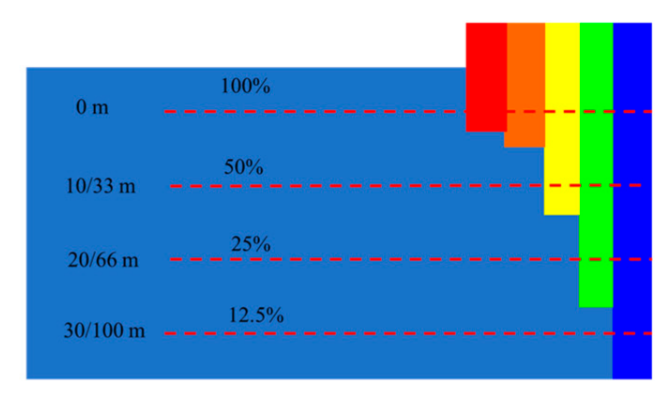
1. Selective Light Absorption
Water acts as a natural color filter. Red wavelengths (620-750 nm) are absorbed within the first 3-5 meters, orange and yellow follow suit at 5-15 meters, leaving only blue-green light to dominate deeper waters. This is why everything looks eerily blue-green below the surface.
2. Light Scattering
Suspended particles like plankton, sediment, and organic matter scatter light in all directions, creating a hazy, low-contrast appearance similar to fog on land. This phenomenon reduces visibility and blurs fine details.
3. Color Cast and White Balance Issues
The absence of a natural white-light reference underwater makes white balance difficult for cameras, often producing images with severe color casts that don’t accurately represent the scene.
2. The Solution: A Multi-Stage Enhancement Pipeline
Our implementation tackles these challenges through a sophisticated six-stage processing pipeline.
- White Balance Correction (LAB color space)
- Red Channel Restoration
- Contrast-Limited Adaptive Histogram Equalization (CLAHE)
- Dehazing via Dark Channel Prior
- Adaptive Unsharp Masking
- Gamma Correction
2.1 White Balance Correction in LAB Color Space
Theory: The LAB color space provides a perceptually uniform representation where L represents lightness, A represents green-red chromaticity, and B represents blue-yellow chromaticity. The gray-world assumption suggests that, on average, a natural image should have neutral colors, meaning the A and B channels are centered around 128 in an 8-bit LAB image.
Implementation: The white_balance function converts to LAB color space to separate luminance from chromaticity, then shifts the A and B channel means back to neutral gray (128). Float32 arithmetic prevents overflow, and user-adjustable shifts enable fine-tuning for different water conditions.
def white_balance(img):
    lab = cv2.cvtColor(img, cv2.COLOR_BGR2LAB)
    L, A, B = cv2.split(lab)
    A = A.astype(np.float32)
    B = B.astype(np.float32)


    A = A - (np.mean(A) - 128) + A_SHIFT
    B = B - (np.mean(B) - 128) + B_SHIFT


    A = np.clip(A, 0, 255).astype(np.uint8)
    B = np.clip(B, 0, 255).astype(np.uint8)


    return cv2.cvtColor(cv2.merge([L, A, B]), cv2.COLOR_LAB2BGR)
2.2 Red Channel Restoration
Theory: Red wavelengths are absorbed first underwater, compressing the red channel’s dynamic range. Histogram equalization redistributes pixel intensities across the full range, revealing hidden details.
Implementation: The restore_red function equalizes the red channel histogram to expand its compressed dynamic range, then blends it with the original using weighted addition. The strength parameter controls the blend ratio, preventing over-amplification of noise while restoring color information.
def restore_red(img):
    b, g, r = cv2.split(img)
    boost = cv2.equalizeHist(r)
    strength = RED_STRENGTH / 100.0
    r_new = cv2.addWeighted(r, 1 - strength, boost, strength, 0)
    return cv2.merge([b, g, r_new])
2.3 Contrast-Limited Adaptive Histogram Equalization (CLAHE)
Theory: Standard histogram equalization amplifies noise in uniform regions. CLAHE partitions the image into tiles, applies local equalization with contrast clipping, and blends boundaries smoothly to prevent tile artifacts.
Implementation: The algorithm works in the LAB color space to enhance only the luminance channel, avoiding color distortion. It creates 8×8 tiles, applies local histogram equalization with contrast clipping, and then blends tile boundaries smoothly to prevent artifacts.
def clahe_enhance(img):
    lab = cv2.cvtColor(img, cv2.COLOR_BGR2LAB)
    L, A, B = cv2.split(lab)
    clahe = cv2.createCLAHE(clipLimit=max(CLAHE_CLIP, 0.1))
    L2 = clahe.apply(L)
    return cv2.cvtColor(cv2.merge([L2, A, B]), cv2.COLOR_LAB2BGR)
2.4 Dehazing via Dark Channel Prior
Theory: The dark channel prior states that clear images have at least one color channel with very low intensity in local patches. Haze/scattering violates this by adding brightness. We estimate atmospheric light from bright pixels, compute a transmission map, and recover the scene radiance.
Implementation: The dehaze function estimates atmospheric light from the brightest 5% of pixels, computes the transmission map, and recovers scene radiance using the image formation model. The T_MIN threshold prevents division instability, while OMEGA controls dehazing strength.
def dehaze(img):
    gray = cv2.cvtColor(img, cv2.COLOR_BGR2GRAY).astype(np.float32)
    A = np.percentile(gray, 95)
    t = 1 - OMEGA * (gray / A)
    t = np.clip(t, T_MIN, 1.0)
    t = cv2.merge([t, t, t])
    J = (img.astype(np.float32) - A) / t + A
    return np.clip(J, 0, 255).astype(np.uint8)
2.5 Adaptive Unsharp Masking
Theory: Unsharp masking enhances edges by subtracting a blurred version: I_sharp = I + α(I – blur). This is equivalent to I_sharp = (1+α)I – α×blur. In this formula, I_sharp represents the sharpened output image, I is the original image, blur is the Gaussian-blurred version, and α (alpha) is the sharpening strength parameter that controls how much of the edge detail is added back.


Implementation: Applies Gaussian blur to extract low-frequency components, then uses weighted addition to create the unsharp mask effect (1.2×original – 0.2×blur), which enhances edge details without creating halos.
def sharpen(img):
    blur = cv2.GaussianBlur(img, (3, 3), 0)
    return cv2.addWeighted(img, 1.2, blur, -0.2, 0)
2.6 Gamma Correction
Theory: Gamma correction applies power-law transformation V_out = 255(V_in/255)^(1/γ). For γ > 1, this brightens shadows more than highlights, improving visibility in darker regions.
Implementation: Precomputes a 256-element lookup table (LUT) for the power-law transformation, enabling O(1) per-pixel operation instead of expensive power computations. The cv2.LUT function applies the table efficiently across all pixels.
def gamma_correct(img, g=1.1):
    inv = 1.0 / g
    table = np.array([(i / 255.0) ** inv * 255 for i in range(256)]).astype("uint8")
    return cv2.LUT(img, table)
3. Real-Time Interactive System using OpenCV HighGUI
Let’s create a GUI application to adjust colors just like we do in Photoshop or similar applications. OpenCV HighGUI provides several interactive controls, such as TrackBars and buttons. Check out this article on OpenCV HighGUI to learn more in-depth.
3.1 Trackbar Callback
Synchronizes global parameters with trackbar positions whenever any slider moves. Trackbar values are scaled to appropriate ranges: [0,100] mapped to −50 to +50 for shifts, [0,100] mapped to 0.0–1.0 for omega, and [0,50] mapped to 0.0–5.0 for the CLAHE clip limit.
def on_trackbar(val):
    global A_SHIFT, B_SHIFT, OMEGA, CLAHE_CLIP, RED_STRENGTH
    try:
        A_SHIFT = cv2.getTrackbarPos("A Shift", "Enhanced") - 50
        B_SHIFT = cv2.getTrackbarPos("B Shift", "Enhanced") - 50
        OMEGA = cv2.getTrackbarPos("Omega", "Enhanced") / 100.0
        CLAHE_CLIP = cv2.getTrackbarPos("CLAHE Clip", "Enhanced") / 10.0
        RED_STRENGTH = cv2.getTrackbarPos("Red Boost", "Enhanced")
    except cv2.error:
        return
3.2 Video Processing
Processes the entire video file frame by frame using the current parameter settings. Extracts video properties (width, height, fps) to maintain consistency in the output file written with the MP4V codec.
out = cv2.VideoWriter("enhanced_video.mp4",cv2.VideoWriter_fourcc(*"mp4v"), fps, (w, h))

    while True:
        ret, frame = cap.read()
        if not ret:
            break
        enhanced = enhance_underwater(frame)
        out.write(enhanced)
3.3 Main Application Loop
Creates side-by-side windows for comparison, initializes trackbars with default values, and runs the main loop. The loop handles mode switching (image/video), applies enhancement in real-time, and saves results on ‘s’ key press. Video mode loops indefinitely for continuous preview.
def run_app(image_path, video_path):

    cv2.namedWindow("Enhanced", cv2.WINDOW_NORMAL)
    cv2.resizeWindow("Enhanced", 900, 900)


    cv2.namedWindow("Original", cv2.WINDOW_NORMAL)
    cv2.resizeWindow("Original", 900, 900)


    img = cv2.imread(image_path)
    img = cv2.resize(img, (900, 900))
3.4 Image and Video Outputs:
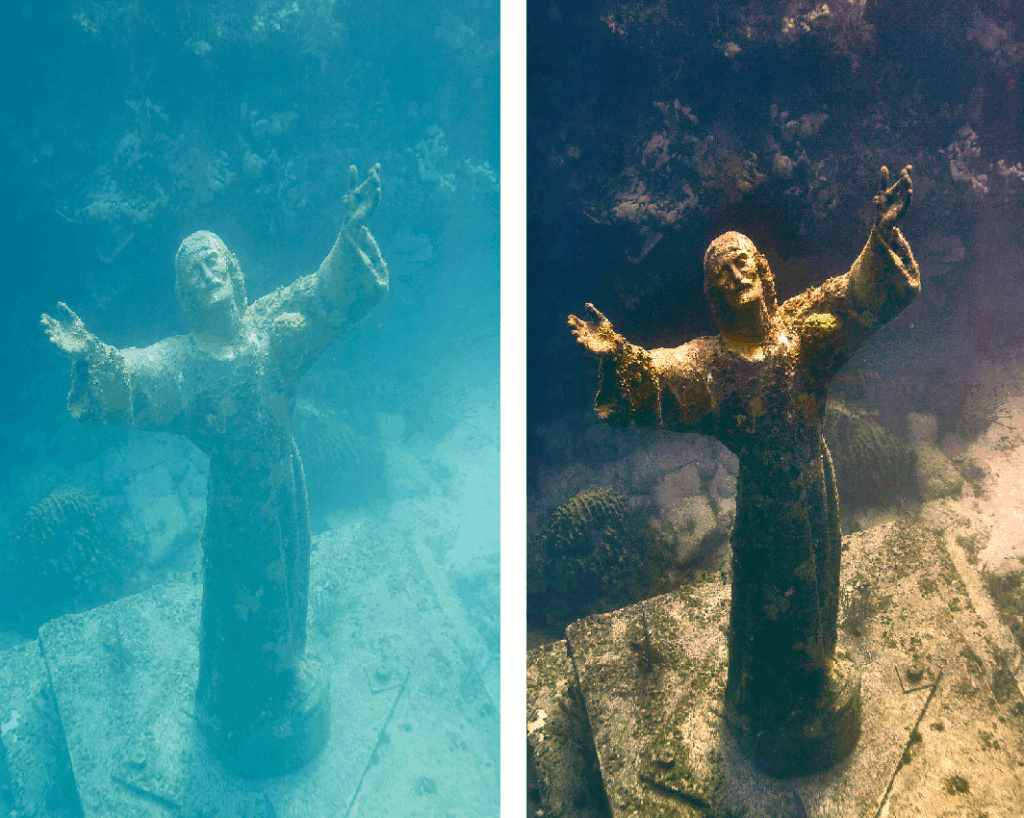
Original image vs Enhanced image
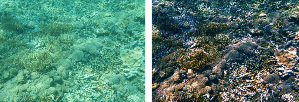
Original image vs Enhanced image
Original Video Input
Enhanced Video Output
4. Working with RAW Underwater Datasets
4.1 Why Use RAW Datasets?
For optimal enhancement results, working with RAW or minimally processed underwater image datasets is strongly recommended over heavily compressed consumer formats. High-quality underwater datasets preserve critical image information that is essential for accurate enhancement. This yields cleaner, more detailed data for the pipeline, enabling stronger corrections without noise amplification or posterization.
4.2 Recommended Datasets
For training or testing the underwater enhancement pipeline, consider using these publicly available datasets:
5. Parameter Guidelines
| Parameter | Range | Default | Effect |
| A_SHIFT | -50 to +50 | 0 | Fine-tune green-red balance |
| B_SHIFT | -50 to +50 | 0 | Fine-tune blue-yellow balance |
| OMEGA | 0.0 to 1.0 | 0.75 | Dehazing strength (higher = more aggressive) |
| CLAHE_CLIP | 0.1 to 5.0 | 1.2 | Contrast enhancement limit (higher = more contrast) |
| RED_STRENGTH | 0 to 100 | 30 | Red channel restoration intensity |
| T_MIN | 0.1 to 0.5 | 0.35 | Minimum transmission (prevents artifacts) |
6. Applications of Underwater Image Enhancement
- Marine Biology Research: Species identification and behavioral analysis in turbid waters
- Underwater Archaeology: Enhanced visibility of artifacts and structural details in excavations
- AUV Navigation: Real-time enhancement for obstacle detection and inspection tasks
- Infrastructure Inspection: Defect detection in underwater pipelines, cables, and offshore platforms
- Scientific Documentation: High-quality imaging for research publications and presentations
7. Conclusion and Key Takeaways
This multi-stage enhancement pipeline demonstrates the effectiveness of combining classical computer vision techniques to address underwater imaging challenges. The modular architecture allows parameter optimization across diverse conditions from clear tropical waters to turbid coastal environments. The OpenCV implementation provides both computational efficiency and accessibility for researchers, engineers, and practitioners.


5K+ Learners
Join Free VLM Bootcamp3 Hours of Learning