

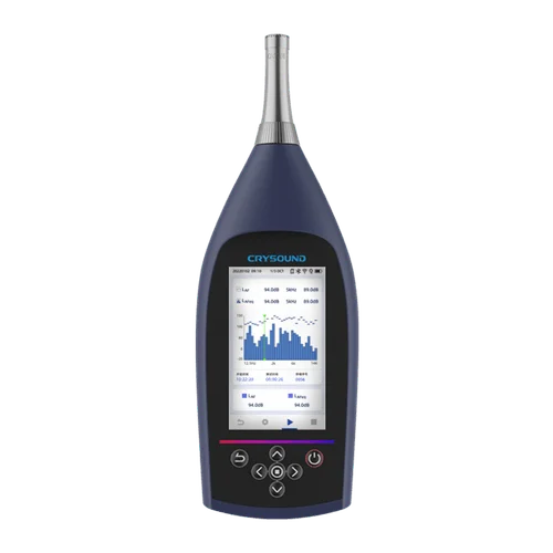
PIONEER THE NEW SOUNDWAVE
CRYSOUND Global New Product Launch
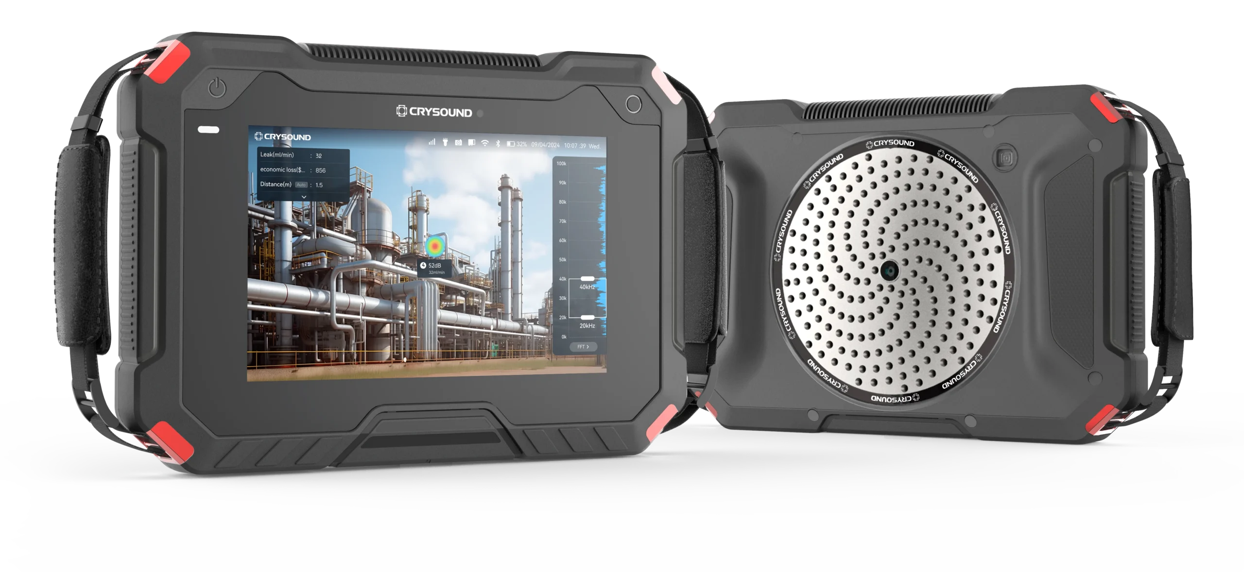
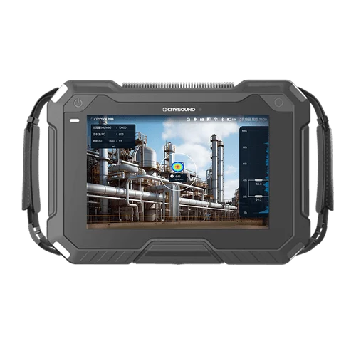
CRY8125 Ex Advanced Acoustic Imaging Camera
Measure Sound Better
Measure Sound Better
At CRYSOUND, precision blends innovation. With over 25 years of expertise in acoustic measurement, we deliver cutting-edge solutions that drive progress from consumer electronics to environmental management. Looking to the future, we are committed to providing world-class acoustic testing equipment while empowering users to be the champions of audio test and detection solutions.
Solutions
Industry leading solutions for accurate acoustic measurements
Gas Leak Detection
CRYSOUND offers a versatile gas leak detection solution for both ordinary and explosion-proof...
Noise and Vibration Test
CRYSOUND conducts noise and vibration tests for diverse environments, encompassing traffic, airport...
Electroacoustic Test
CRYSOUND's electroacoustic test solutions are tailored to assess a wide range of consumer...
Blog
Company News, Case Study

AR Glasses Production-Line Testing Upgrade – Multi-Station Audio & VPU Solution
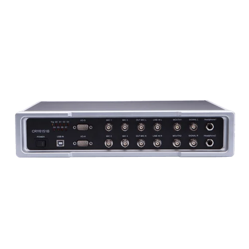
As the AR glasses market transitions from proof-of-concept to large-scale commercialization, product capabilities in audio and haptic interaction continue to expand, driving increased demands for production-line testing. With key modules such as audio and VPU (Vibration Processing Units), AR glass production-line testing is evolving from simple functional validation to consistency control aimed at enhancing real-world user experience. Based on actual mass production project experience, this article introduces audio and VPU testing solutions for different workstations, with a focus on free-field audio testing, VPU deployment, and fixture design, providing practical reference for scaling AR glasses manufacturing. Accelerating Market Expansion of AR Glasses and New Trends in Production-Line Testing As smart glasses products mature, their functional boundaries are expanding rapidly. According to various industry reports, the shipment volume and investment scale of AR glasses continue to increase, with the market shifting from concept validation to commercialization. Products driven by companies like Meta are increasingly capable of supporting voice interaction, calls, notifications, and recording, supplementing functions traditionally carried out by smartphones and earphones. This shift has transformed AR glasses from a low-frequency conceptual product into a high-frequency wearable interaction terminal. Consequently, audio capabilities have become a core component of the smart glasses experience, directly impacting voice interaction and call quality. At the same time, vibration and haptic feedback have been introduced to enhance interaction confirmation and user perception. As these capabilities become commonplace in mass-produced products, production-line testing is no longer just focused on whether basic functions work but is now required to handle multiple critical capabilities, such as audio and VPU, simultaneously. This shift presents new challenges for upgrading production-line testing solutions. Audio Testing Solutions for Multi-Station Production Lines Audio is one of the most directly influential functions on the user experience of AR glasses, and its production-line testing needs to balance accuracy, consistency, and production efficiency. In a multi-station production environment, audio testing is often distributed across several workstations depending on the assembly phase. At the temple or frame workstations, audio testing focuses more on validating the basic performance of individual microphones or speakers, ensuring that key components meet the requirements early in the assembly process and avoiding costly rework later on in the process. At the final assembly workstation, the focus shifts to overall audio performance and system-level coordination. While different workstations focus on different aspects, the fixture positioning, acoustic environment control, and testing process design need to maintain consistent logic throughout. CRYSOUND’s AR glass audio testing solutions are designed to address this need, with a unified testing architecture that allows flexible deployment across different workstations while maintaining stable and consistent results. The solutions can be divided into the following two types, meeting the aesthetic and UPH requirements of different production lines. Drawer-Type Single-Unit (1-to-1) Easy automation integration Standing operation for convenient loading and unloading Simultaneous testing of SPK and MIC (airtightness), supporting multi-MIC scenarios Serial testing for left and right SPK, parallel testing for multiple MICs Supports Bluetooth, USB ADB, and Wi-Fi ADB communication Average cycle time (CT): 100s | UPH: 36 Clamshell Dual-Unit (1-to-2) Parallel dual-unit testing for improved efficiency Ergonomic seated operation design Simultaneous testing of SPK and MIC (airtightness), supporting multi-MIC scenarios Serial testing for left and right SPK (single box), parallel testing for multiple MICs Supports Bluetooth, USB ADB, and Wi-Fi ADB communication Average cycle time (CT): 150s | UPH: 70 Speaker EQ in AR Glasses: From Pressure Field to Free Field In traditional earphone products, speaker EQ is usually built in a relatively stable pressure-field environment, where ear coupling and wearing style have a well-controlled impact on the acoustic environment. In contrast, AR glasses typically use open structures for the speakers, with no sealed cavity between the driver and the ear, making their acoustic performance closer to free-field characteristics. This structural difference makes the frequency response of AR glasses speakers more sensitive to sound radiation direction, structural reflections, and wearing posture, and dictates that their EQ strategy cannot simply follow earphone product experience. In the production-line testing and tuning process, the speaker EQ for AR glasses needs to be evaluated and validated under free-field conditions. Due to the open acoustic structure, the frequency response is more susceptible to structural reflections, assembly tolerances, and variations in wearing posture, making it difficult to rely solely on hardware consistency to ensure stable listening across different products. By introducing EQ tuning, these systemic deviations can be compensated without changing the structural design, improving the consistency of audio performance during mass production. The focus of the testing solution is not to pursue idealized sound quality, but rather to capture real acoustic differences under stable and repeatable free-field testing conditions, providing reliable data for EQ parameter validation. CRYSOUND supports customized EQ algorithms. In one mass production project, speaker EQ calibration was introduced at the final test station under free-field conditions, and the results were accepted by the customer, validating the applicability and practical significance of this solution for glasses products. VPU Testing Solutions for AR/Smart Glasses Why AR Glasses Include VPU (Vibration Processing Unit) As AR/smart glasses increasingly support voice interaction, calls, and notifications, relying on audio feedback alone is no longer enough. In noisy environments, privacy-sensitive scenarios, or with low-volume prompts, users need a feedback method that does not disturb others but is sufficiently clear. This is where VPU is introduced. Unlike traditional earphones, glasses are not always tightly coupled to the ear, making audio prompts more susceptible to environmental noise. By utilizing vibration or haptic feedback, the system can convey status confirmations, interaction responses, or notifications to users without increasing volume or relying on screens. Therefore, VPU becomes a key component for supplementing or even replacing some audio feedback in AR glasses. Primary Roles of VPU in AR Glasses In current mass-produced smart glasses designs, VPU typically serves the following functions: Interaction confirmation feedback: such as successful voice wake-up, completed command recognition, or the start/stop of recording or photo taking. Silent notifications: vibrational feedback in scenarios where audio prompts are unsuitable. Enhanced experience: boosting interaction certainty and immersion when combined with audio feedback. These functions have made VPU an essential capability in the AR glasses interaction experience, rather than just an optional feature. Typical VPU Placement in AR Glasses (Why in the Nose Bridge/Pads) Structurally, VPU is typically located near the nose bridge or nose pads for three main reasons: Proximity to sensitive body areas: The nose bridge is sensitive to small vibrations, providing high feedback efficiency. Stable and consistent coupling: Compared to the temples, the nose bridge has a more stable and consistent contact with the face, ensuring better vibration transmission. Does not interfere with audio device layout: Avoids interference with speakers and microphones in the temple region. Therefore, during production-line testing, VPU is often tested as an independent target, requiring dedicated verification at the frame or final assembly stage. VPU Testing Implementation and Consistency Control on the Production Line Based on the functional positioning and structural characteristics of VPU in AR glasses, VPU testing is typically scheduled based on the product form and assembly progress in mass production. In some cases, testing may even be moved earlier in the process to identify potential VPU issues before they are exacerbated in subsequent assembly stages. It is important to note that production-line testing environments differ fundamentally from laboratory validation environments. In laboratory testing, VPU is typically tested as a standalone component under simplified conditions and higher excitation levels (e.g., 1g). However, in production-line environments, the VPU is already integrated into the frame or complete product, requiring excitation conditions that closely mimic those of real-world wearing scenarios. In practice, production-line VPU testing typically takes place in the 0.1g–0.2g, 100–2kHz excitation range, verifying consistency in VPU performance under realistic physical conditions. CRYSOUND’s AR glasses VPU production-line testing solution uses the CRY6151B Electro-Acoustic Analyzer as the testing and analysis platform. The vibration table provides stable excitation, and the product VPU synchronizes vibration response signals with a reference accelerometer. Software analysis evaluates key parameters such as frequency response (FR) and total harmonic distortion (THD).This test architecture balances testing effectiveness and production-line throughput, meeting the deployment needs for VPU testing at different stations. Compared to audio testing, VPU testing is more sensitive to testing configurations and fixture design, with less room for error and greater difficulty in consistency control. Based on experience from multiple projects, fixture design must fully account for structural differences in locations such as the nose bridge and nose pads. It is important to prioritize materials and contact methods that facilitate vibration transmission, and to design standardized fixture shapes that keep the fixture's center of gravity aligned with the vibration table's working plane, minimizing the introduction of additional variables at the structural level. By following these design principles, the stability and repeatability of VPU test results can be improved in a production-line environment, providing reliable support for validating the product's VPU capabilities. From Functional Testing to Experience Constraints In AR glasses production lines, the role of testing is evolving. In the past, audio or vibration modules were more likely to be treated as independent functions, with the goal of confirming whether they were "functional." However, with the current form of the product, these modules directly influence voice interaction, wearing comfort, and overall experience. As a result, the test results now serve as a prerequisite for the overall product performance. For example, audio and VPU modules are no longer just performance verification items; they now play a role in the consistency control of the user experience. The interaction between audio performance, vibration feedback, and structural assembly means that production-line testing needs to identify potential issues that could affect the experience in advance, rather than just filtering out problems at the final inspection stage. This change is pushing test strategies from "functional pass" to "experience control." If you’d like to learn more about AR glasses audio testing solutions—or discuss your blade process and inspection targets—please use the “Get in touch” form below. Our team can share recommended settings and an on-site workflow tailored to your production conditions.

Octave-Band Analysis Guide: FFT Binning vs. Filter Bank Method
Octave-band analysis can be implemented in two fundamentally different ways: FFT binning (integrating PSD/FFT bins into 1/1- and 1/3-octave bands) and a true octave filter bank (standards-oriented bandpass filters + RMS/Leq averaging). In this post, we compare how the two methods work, where their results match, where they diverge (scaling, window ENBW, band-edge weighting, latency, transient response), and how OpenTest supports both for acoustics, NVH, and compliance measurement. For a detailed explanation of the concepts, read this → Octave-Band Analysis: The Mathematical and Engineering Rationale Octave-band filter banks (true octave / CPB filter bank) Parallel bandpass filters + energy detector + time averaging A filter-bank (true octave) analyzer typically: Design a bandpass filter H_b(z) (or H_b(s)) for each band center frequency. Run filters in parallel to obtain band signals y_b(t). Compute band mean-square/power and apply time averaging to output band levels. To be comparable across instruments, filter magnitude responses must satisfy IEC/ANSI tolerance masks (class) for the specified filter set. [1][3] IIR vs FIR: why IIR (cascaded biquads) is common in practice IIR advantages: lower order for a given roll-off, lower compute, good for real-time/embedded; stable when implemented as SOS/biquads. FIR advantages: linear phase is possible (useful when waveform shape matters); design/verification can be more straightforward. For band-level outputs, phase is usually not the primary concern, so IIR filter banks are common. Multirate processing: the “secret weapon” of CPB filter banks Low-frequency CPB bands are very narrow. Implementing them at the full sampling rate is inefficient. A common strategy is to group bands by octave and downsample for low-frequency groups: Low-pass then decimate (e.g., by 2 per octave) for lower-frequency groups. Implement the corresponding bandpass filters at the reduced sampling rate. Ensure adequate anti-aliasing before decimation. Time averaging / time weighting: band levels are statistics, not instantaneous values Band levels typically require time averaging. Common options include block RMS, exponential averaging, or Leq (energy-equivalent level). In sound level meter contexts, IEC 61672-1 defines Fast/Slow time weightings (Fast ~125 ms, Slow ~1 s). [5][6] Engineering implication: different time constants produce different readings, so time weighting must be stated in reports. How to validate that a filter bank behaves “like the standard” Sine sweep: verify passband behavior and adjacent-band isolation; observe time delay effects. Pink/white noise: verify average band levels and variance/stabilization time; check effective bandwidth behavior. Impulse/step: examine ringing and time response (critical for transient use). Cross-check against a known compliant reference instrument/implementation. From band definitions to compliant digital filters: an end-to-end workflow (conceptual) Choose the band system: base-10/base-2, the fraction 1/b (commonly b=3), generate exact fm and f1/f2. Choose performance target: which standard edition and which class/mask tolerance? Choose filter structure: IIR SOS for real-time; FIR or forward-backward filtering if phase/zero-phase is required. Design each bandpass: map f1/f2 into the digital domain correctly (e.g., pre-warp for bilinear transform). Implement multirate if needed: decimate for low-frequency groups with sufficient anti-alias filtering. Verify: magnitude response vs mask; noise tests for effective bandwidth; sweep/impulse tests for time response. Calibrate and report: units and reference quantities, averaging/time weighting, method details. Time response explained: group delay, ringing, and averaging all shape readings A band-level analyzer is a time-domain system (filter → energy detector → smoother), so readings are governed by multiple time scales: Filter group delay: how late events appear in each band. Filter ringing/decay: how long a short pulse “rings” within a band. Energy averaging/time weighting: the time resolution vs fluctuation of the output level. Thus, for transients (impacts, start/stop events, sweeps), different compliant implementations can yield different peak levels and time tracks—consistent with ANSI’s caution. [3] Rule of thumb: for steady-state contributions, use longer averaging for stability; for transient localization, shorten averaging but accept higher variability and lock down algorithm details. Common real-time pitfalls Forgetting anti-aliasing in the decimation chain: low-frequency bands become contaminated by aliasing. Numerical instability of high-Q low-frequency IIR sections: use SOS/biquads and sufficient precision. Averaging in dB: always average in energy/mean-square, then convert to dB. Assuming band energies must sum exactly to total energy: standard filters are not necessarily power-complementary; verify using standard-consistent criteria instead. Octave-Band Filter Bank Analysis in OpenTest OpenTest supports octave-band analysis using a filter-bank approach:1) Connect the device, such as SonoDAQ Pro2) Select the channels and adjust the parameter settings. For an external microphone, enable IEPE and switch to acoustic signal measurement.3) In the Octave-Band Analysis section under Measurement Mode, choose the IEC 61260-1 algorithm. It supports real-time analysis, linear averaging, exponential averaging, and peak hold.4) After configuring the parameters, click the Test button to start the measurement.5) A single recording can be analyzed simultaneously in 1/1-octave, 1/3-octave, 1/6-octave, 1/12-octave, 1/24-octave, and 1/24-octave bands. Figure 1: Octave-Band Filter Bank Analysis in OpenTest FFT binning and FFT synthesis FFT binning: convert a narrowband spectrum into CPB band integrals Estimate spectrum (single FFT, Welch PSD, or STFT). Integrate/sum within each octave/fractional-octave band to obtain band power. This is common in software/offline work because a single FFT provides high-resolution spectrum that can be re-binned into any band system (1/1, 1/3, 1/12, …). Key challenge #1: FFT scaling and window corrections After an FFT, scaling depends on your definitions: 1/N normalization, amplitude vs power vs PSD, one-sided vs two-sided spectrum, and windowing. For noise measurements, ENBW is crucial; ignoring it can introduce systematic offsets. [7] A practical PSD normalization (periodogram form) # convert to one-sided PSD: multiply by 2 except DC (and Nyquist if present) This yields PSD in units of (input unit)²/Hz and supports energy consistency checks by integrating PSD over frequency. Two quick self-checks for scaling White noise check: generate noise with known variance σ²; integrate one-sided PSD over 0..fs/2 and recover ≈σ² (accounting for the ×2 rule). Pure tone check: generate a sine with amplitude A (RMS=A/√2); integrating spectral energy should recover ≈A²/2 (subject to leakage and window choice). If both checks pass, your FFT scaling is likely correct; then partial-bin weighting and octave binning become meaningful. Key challenge #2: band edges rarely align to bins → partial-bin weighting Hard include/exclude decisions at band edges cause step-like errors, especially at low frequency where bands are narrow. Use overlap-based weighting (Section 4.2.4) for the boundary bins. Does zero-padding solve edge misalignment? (common misconception) Zero-padding interpolates the displayed spectrum but does not improve true frequency resolution (which is set by the original window length). It can reduce visual stair-stepping but cannot turn 1–2-bin low-frequency bands into reliable band-level estimates. Fundamental fixes are longer windows or multirate processing/filter banks. Key challenge #3: time–frequency trade-off (window length sets low-frequency accuracy and delay) FFT resolution is Δf = fs/N. Low-frequency 1/3-octave bands can be only a few Hz wide, so achieving enough bins per band requires very large N, increasing latency and smoothing transients. Root cause: 1/3 octave is constant-Q, but STFT uses constant-Δf bins In CPB, band width scales with frequency (Δf_band ∝ f, constant-Q). In STFT, bin spacing is constant (Δf_bin constant). Therefore low-frequency CPB needs extremely fine Δf_bin (long windows), while high frequency is over-resolved. Solution routes: long-window STFT vs multirate STFT vs CQT/wavelets Long-window STFT: simplest, but high latency and transient smearing. Multirate STFT: downsample low-frequency content and FFT at lower fs, similar in spirit to multirate filter banks. Constant-Q transform (CQT) / wavelets: naturally logarithmic resolution, but matching IEC/ANSI masks requires extra calibration/validation. [4] For compliance measurements, standards-oriented filter banks are preferred; for research/feature extraction, CQT/wavelets can be attractive. FFT synthesis: constructing per-band filtering in the frequency domain FFT synthesis pushes the FFT approach closer to a filter bank: Define a frequency-domain weight W_b[k] per band (brick-wall or smooth/mask-like). Compute Y_b[k] = X[k]·W_b[k] and IFFT to get y_b[n]. Compute band RMS/averages from y_b[n]. It can easily implement zero-phase (non-causal) filtering. For strict IEC/ANSI matching, W_b and normalization must be carefully designed and validated. Making FFT synthesis stream-like: OLA, dual windows, and amplitude normalization To output continuous time signals per band, use overlap-add (OLA): frame, window, FFT, apply W_b, IFFT, synthesis window, and OLA. Choose analysis/synthesis windows to satisfy COLA (constant overlap-add) conditions (e.g., Hann with 50% overlap) to avoid periodic level modulation. If the goal is to match standard filters, how should W_b be chosen? W_b[k] depends on what you want to match: Match brick-wall integration: W_b is hard 0/1 within [f1,f2]. Match IEC/ANSI filter behavior: |W_b(f)| approximates the standard mask and effective bandwidth (matches ∫|W_b|²). Match energy complementarity for reconstruction: design Σ_b |W_b(f)|² ≈ 1 (Section 7.6). You typically cannot satisfy all three perfectly at once; define your priority (compliance vs decomposition/reconstruction) up front. Energy-conserving frequency-domain filter banks: why Σ|W_b|² matters If you want band energies to sum to total energy (within numerical error), a common design aims for approximate power complementarity: IEC/ANSI masks do not necessarily enforce strict complementarity, so don’t assume exact additivity in compliance contexts. Welch/averaging strategies: how to make FFT band levels stable Use Welch averaging (segment, window, overlap, average power spectra). Average in the power domain (|X|² or PSD), then convert to dB. For non-stationary signals, consider STFT to obtain time–band matrices. Report window type, overlap, averaging count, and ENBW/CG treatment. FFT-Binning Analysis in OpenTest OpenTest supports octave-band analysis based on FFT binning:1) Connect the device, such asSonoDAQ Pro2) Select the channels and adjust the parameter settings. For an external microphone, enable IEPE and switch to acoustic signal measurement.3) In the Octave-Band Analysis section under Measurement Mode, choose the FFT-based algorithm.4) A single recording can be analyzed simultaneously in 1/1-octave, 1/3-octave, 1/6-octave, 1/12-octave, and 1/24-octave bands. Figure 2: FFT-Binning Octave-Band Analysis in OpenTest Filter-bank vs FFT/FFT synthesis: differences, equivalence conditions, and trade-offs A comparison table DimensionFilter-bank (True Octave / CPB)FFT binning / FFT synthesisStandards complianceEasier to match IEC/ANSI magnitude masks; mainstream for hardware instruments. [1][3]Hard binning behaves like band integration; matching masks requires extra weighting or standard-compliant digital filters.Real-time / latencyCausal real-time possible; latency set by filter order and averaging.Block processing adds at least one window length of delay; low-frequency resolution often forces longer windows.Transient responseContinuous output but affected by group delay/ringing; different compliant implementations may differ. [3]Set by STFT windowing; transients are smeared by windows and sensitive to window type/length.Leakage & correctionsControlled via filter design; leakage can be managed.Strongly depends on window and ENBW/scaling; edge-bin misalignment needs partial weighting. [7]InterpretabilityRMS after bandpass filtering—aligned with sound level meters and analyzers.Spectrum estimation + binning—more statistical; interpretation depends on window/averaging settings.ComputationMany filters in parallel; multirate can reduce cost.One FFT can serve all bands; efficient for offline/batch.Phase & reconstructionIIR is typically nonlinear phase (fine for levels).Frequency weights can be zero-phase; reconstruction needs attention to complementarity and transitions. When do both methods give (almost) the same answers? Band-averaged results typically agree closely when: You compare averaged band levels (not transient peak tracks). The signal is approximately stationary and the observation time is long enough. FFT resolution is fine enough that each band contains enough bins (especially at the lowest band). FFT scaling is correct (one-sided handling, Δf, window U, ENBW/CG where needed). Partial-bin weighting is used at band edges. Why differences grow for transients and short events Differences are driven by mismatched time scales: filter banks have band-dependent group delay and ringing but continuous output; STFT uses a fixed window that sets both frequency resolution and time smoothing. If event duration is comparable to the window length or filter impulse response, results depend strongly on implementation details. Error budget: where mismatches usually come from (and how to locate them quickly) Wrong averaging/combination in dB: must average and sum in the energy domain. Inconsistent FFT scaling: 1/N conventions, one-sided vs two-sided, Δf, window normalization U. Missing window corrections: ENBW for noise; coherent gain/leakage for tones. Using nominal frequencies to compute edges instead of exact definitions. No partial-bin weighting at band boundaries (especially harmful at low frequency). Multirate/anti-alias issues in filter banks. Different averaging time constants/windows between methods. True method differences: brick-wall binning vs standard filter skirts/roll-off imply systematic offsets. A strong debugging approach: first match total mean-square using white noise (scaling/ENBW/partial-bin), then validate band centers and adjacent-band isolation using swept sines or tones. Engineering checklist: make 1/3-octave analysis correct, stable, and reproducible Choose a method: compliance → filter bank; offline statistics → FFT binning For regulations/type testing/instrument comparability: prefer IEC/ANSI-compliant filter banks and report standard edition and class. [1][3] For offline processing, large datasets, or flexible band definitions: FFT binning can be efficient, but scaling and boundary weighting must be rigorous. If you need per-band time-domain signals (modulation, envelope, etc.): consider FFT synthesis or explicit filter banks. Selecting FFT parameters from the lowest band (example) Example: fs=48 kHz, lowest band of interest is 20 Hz (1/3 octave). Its bandwidth is only a few Hz. If you want at least M=10 bins per band, you may need Δf_bin ≤ bandwidth/10, implying a very large N (e.g., ~100k points; 2^17=131072). This illustrates why real-time compliance often favors filter banks. Typical mistakes that prevent results from matching Summing magnitude |X| instead of power |X|² or PSD. Averaging in dB instead of in linear power/mean-square. Ignoring ENBW/window scaling for noise. [7] Computing band edges from nominal frequencies. Not stating time weighting/averaging conventions (Fast/Slow/Leq). [5][6] Recommended validation flow (regardless of implementation) Tone-at-center test (or sweep): verify that energy peaks in the correct band and adjacent-band rejection behaves as expected. White/pink noise: verify expected spectral shape in band levels and assess stability/averaging time. Cross-implementation comparison: compare your implementation with a known reference on identical signals; isolate scaling vs definition vs filter-skirt differences. Record and freeze parameters (band definition, windowing, averaging) in the test report. Reproducibility checklist: include these in reports so others can recompute your levels Band definition: base-10 or base-2? b in 1/b? exact vs nominal used for computation? reference frequency fr? Implementation: standard filter bank (IIR/FIR, multirate) vs FFT binning/synthesis; software/library versions. Sampling/preprocessing: fs, detrending/DC removal, anti-alias filtering, resampling. Time averaging: Leq / block RMS / exponential; time constants, block size, overlap, averaging frames; Fast/Slow context if relevant. FFT details (if used): window type, N, hop, zero-padding, PSD normalization, one-sided handling, ENBW/CG, partial-bin weighting. Calibration/units: input units and reference quantities (e.g., 20 µPa), sensor calibration factors and dates. Output definition: RMS vs peak vs band power; 10log vs 20log conventions; any band aggregation steps. If you remember one line: document “band definition + time averaging + FFT scaling/window treatment (if any)”. Most disputes disappear. Quick formulas and numeric example (ready for code/report) Base-10 one-third-octave constants G = 10^(3/10) ≈ 1.995262 r = 10^(1/10) ≈ 1.258925 # adjacent center-frequency ratio k = 10^(1/20) ≈ 1.122018 # edge multiplier about center f1 = fm / k f2 = fm * k Example: the 1 kHz one-third-octave band fm = 1000 Hz f1 = 1000 / 1.122018 ≈ 891.25 Hz f2 = 1000 * 1.122018 ≈ 1122.02 Hz Δf ≈ 230.77 Hz Q ≈ 4.33 OpenTest integrates both methods. Download and get started now -> or fill out the form below ↓ to schedule a live demo. Explore more features and application stories at www.opentest.com. References [1] IEC 61260-1:2014 PDF sample (iTeh): https://cdn.standards.iteh.ai/samples/13383/3c4ae3e762b540cc8111744cb8f0ae8e/IEC-61260-1-2014.pdf [3] ANSI S1.11-2004 preview PDF (ASA/ANSI): https://webstore.ansi.org/preview-pages/ASA/preview_ANSI%2BS1.11-2004.pdf [4] HEAD acoustics Application Note: FFT - 1/n-Octave Analysis - Wavelet (filter bank description): https://cdn.head-acoustics.com/fileadmin/data/global/Application-Notes/SVP/FFT-nthOctave-Wavelet_e.pdf [5] IEC 61672-1:2013 (IEC page): https://webstore.iec.ch/en/publication/5708 [6] NTi Audio Know-how: Fast/Slow time weighting (IEC 61672-1 context): https://www.nti-audio.com/en/support/know-how/fast-slow-impulse-time-weighting-what-do-they-mean [7] MathWorks: ENBW definition example: https://www.mathworks.com/help/signal/ref/enbw.html

Octave-Band Analysis: The Mathematical and Engineering Rationale
Octave-band analysis converts detailed spectra into standardized 1/1- and 1/3-octave bands using constant-percentage bandwidth on a logarithmic frequency axis. In this post, we explain the mathematical basis of CPB, why IEC 61260-1 and ANSI S1.11 define octave bands the way they do, and how band levels are computed in practice (FFT binning vs. filter-bank RMS). The goal: repeatable, comparable results for acoustics, NVH, and compliance measurements. What is octave-band analysis, and what problem does it solve? Octave-band analysis is a family of spectrum analysis methods that partition the frequency axis on a logarithmic scale into band-pass bands. Each band has a constant ratio between its upper and lower cut-off frequencies (constant percentage bandwidth, CPB). Within each band we ignore fine line-spectrum details and focus on total energy / RMS (or power) in that band. In other words, it is not “what happens at every 1 Hz,” but “how energy is distributed across equal relative bandwidths.” This representation naturally matches human hearing and many engineering systems, whose frequency resolution is often closer to a relative (log) scale than a fixed-Hz scale. It is a common reporting format required by many standards: room acoustics parameters, sound insulation ratings, environmental noise, machinery noise, wind/road noise, etc., often use 1/3-octave bands. From linear Hz to log frequency: why CPB looks more like an engineering language Using equal-width frequency bins (e.g., every 10 Hz) to accumulate energy leads to inconsistent behavior across the spectrum: At low frequencies, a 10 Hz bin may be too wide and can smear details. At high frequencies, a 10 Hz bin may be too narrow, giving higher variance and less stable estimates for random noise. In contrast, CPB bandwidth grows with frequency (Δf ∝ f). Each band covers a similar relative change, improving stability and repeatability—important for standardized testing. A visual intuition: bandwidth increases on a linear axis, but is uniform on a log axis Figure 1: the same 1/3-octave bands plotted on a linear frequency axis—bandwidth appears larger at high frequencies Each horizontal segment represents a 1/3-octave band [f1, f2]; the short vertical mark is the band center frequency fm. On a linear axis, higher-frequency bands look wider. Figure 2: the same bands on a logarithmic frequency axis—bands become evenly spaced (the essence of CPB) Once the horizontal axis is logarithmic, these bands appear equal-width/equal-spacing; this is exactly what “constant percentage bandwidth” means. These two figures capture the core idea: octave-band analysis uses equal steps on a log-frequency scale, not equal steps in Hz. Standards and terminology: what do IEC/ANSI/ISO systems actually specify? In practice, “doing 1/3-octave analysis” is constrained by more than just band edges. Standards specify (or strongly imply): how center frequencies are defined (exact vs nominal), the octave ratio definition (base-10 vs base-2), filter tolerances/classes, and even the measurement/averaging conventions used to form band levels. IEC 61260-1:2014 highlights: base-10 ratio, reference frequency, and center-frequency formulas IEC 61260-1:2014 is a key specification for octave-band and fractional-octave-band filters. It adopts a base-10 design: the octave frequency ratio is G = 10^(3/10) ≈ 1.99526 (very close to 2, but not exactly 2). The reference frequency is fr = 1000 Hz. It provides formulas for the exact mid-band (center) frequencies and specifies that the geometric mean of band-edge frequencies equals the center frequency. [1] Key formulas (rearranged from the standard): [1] If the fractional denominator b is odd (e.g., 1, 3, 5, ...): If b is even (e.g., 2, 4, 6, ...): And always: Why does the even-b case look “half-step shifted”? Intuitively, the center-frequency grid is evenly spaced on log(f). When b is even, IEC chooses a half-step offset relative to fr so that band edges align more neatly in common reporting conventions. In practice, a robust implementation is to generate the exact fm sequence using the standard’s formula, then compute edges via f1 = fm / G^(1/(2b)) and f2 = fm * G^(1/(2b)), and only then label bands by the usual nominal frequencies. View the data with OpenTest (IEC 61260-1 Octave-Band Analysis) -> Band edges, center frequency, and the bandwidth designator b Standards commonly use 1/b as the “bandwidth designator”: 1/1 is one octave, 1/3 is one-third octave, etc. [1] Once (G, b, fr) are chosen, the entire band set (centers and edges) is fixed mathematically. Exact vs nominal: why two “center frequencies” appear for the same band “Exact” center frequencies are used for mathematically consistent definitions and filter design; “nominal” values are used for labeling and reporting. [1] ISO 266:1997 defines preferred frequencies for acoustics measurements based on ISO 3 preferred-number series (R10), referenced to 1000 Hz. [2] As a result, the exact geometric sequence is typically labeled with familiar nominal values such as: 20, 25, 31.5, 40, 50, 63, 80, 100, 125, 160, …, 1k, 1.25k, 1.6k, 2k, 2.5k, 3.15k, …, 20k. Implementation tip: compute edges from exact frequencies; only round/display as nominal. This avoids drifting away from the standard. Base-10 vs base-2: why standards don’t insist on an exact 2:1 octave Although “octave” is often thought of as 2:1, IEC 61260-1 specifies base-10 (G=10^(3/10)) rather than G=2. Key motivations include: Alignment with decimal preferred-number series (ISO 266 is tied to R10). [2] International consistency: IEC 61260-1:2014 specifies base-10 and notes that base-2 designs are less likely to remain compliant far from the reference frequency. [1] In base-10, one-third octave corresponds to 10^(1/10) ≈ 1.258925 (also interpretable as 1/10 decade), which yields a clean mapping: 10 one-third-octave bands per decade. “10 one-third-octave bands = 1 decade”: why this matters With base-10 one-third-octave spacing, each step multiplies frequency by r = 10^(1/10). Therefore: 10 consecutive 1/3-octave bands multiply frequency by exactly 10 (one decade). This matches ISO 266/R10 conventions and simplifies tables, plotting, and communication. Standardization values readability and consistency as much as raw mathematical purity. Figure 3: Base-10 one-third-octave spacing—10 equal ratio steps per decade (×10 in frequency) ANSI S1.11 / ANSI/ASA S1.11: tolerance classes and a transient-signal caution ANSI S1.11 (and later ANSI/ASA adoptions aligned with IEC 61260-1) specify performance requirements for filter sets and analyzers, including tolerance classes (often class 0/1/2 depending on edition). [3][4] A practical caution in ANSI documents: for transient signals, different compliant implementations can produce different results. [3] This highlights that time response (group delay, ringing, averaging time constants) matters for transient analysis. What do class/mask/effective bandwidth actually control? “I used 1/3-octave bands” is not just about nominal band edges. Standards aim to ensure different instruments/algorithms yield comparable results by constraining: Frequency spacing: center-frequency sequence and edge definitions (base-10, exact/nominal, f1/f2). Magnitude response tolerance (mask): allowable ripple near passband and required attenuation away from center. Energy consistency for broadband noise: constraints on effective bandwidth so band levels are comparable across implementations. Effective bandwidth matters because real filters are not ideal brick walls. For broadband noise, the output energy depends on ∫|H(f)|^2 S(f)df. Differences in passband ripple, skirts, and roll-off can cause systematic offsets. Standards constrain effective bandwidth to keep such offsets within acceptable limits. [1][3][4] The transient caution is not a contradiction: masks mainly constrain steady-state frequency-domain behavior, while transients depend on phase/group delay, ringing, and time averaging. [3] Mathematics: band definitions, bandwidth, Q, and band indexing CPB and equal spacing on a log axis CPB is equivalent to equal-width spacing in log-frequency. If u = log(f), then every band spans a fixed Δu. Many spectra (e.g., 1/f-type) look smoother and statistically more stable in log frequency. Band-edge formulas from the geometric-mean definition (general 1/b form) IEC defines the center frequency as the geometric mean of the edges: fm = sqrt(f1 f2). [1] For 1/b octave bands, the edge ratio is typically f2/f1 = G^(1/b), where G is the octave ratio. Then: For base-10 one-third octave (b=3): G=10^(3/10). Adjacent center ratio is r = G^(1/3) = 10^(1/10) ≈ 1.258925; edge multiplier is k = 10^(1/20) ≈ 1.122018. Q-factor and resolution: octave analysis is constant-Q analysis Define Q = fm / (f2 − f1). For CPB bands, Δf = f2 − f1 scales with fm, so Q depends only on b and G (not on frequency). Quick reference (base-10, fr=1000 Hz): Fractional-octaveBand ratio f2/f1Relative bandwidth Δf/fmQ = fm/Δf1/11.9952620.7045921.4191/21.4125380.3471072.8811/31.2589250.2307684.3331/61.1220180.1151938.6811/121.0592540.05757317.369 Interpretation: for 1/3 octave, Q≈4.33 and each band is about 23% wide relative to its center. Finer bands (1/6, 1/12) give higher resolution but higher variance for random noise and typically require longer averaging. Band numbering (integer index) and formulaic enumeration Implementations often use an integer band index x. In IEC, x appears directly in the center-frequency formula: fm = fr * G^(x/b). [1] This provides a stable way to enumerate all bands covering a target frequency range and ensures contiguous, standard-consistent edges. For base-10: so and you can invert as Figure 4: Q factor for common fractional-octave bandwidths (base-10 definition) Two meanings of “1/3 octave”: base-2 vs base-10—do not mix them Some literature uses base-2: adjacent centers are 2^(1/3). IEC 61260-1 and much modern acoustics practice use base-10: adjacent centers are 10^(1/10). A quick check: if nominal centers look like 1.0k → 1.25k → 1.6k → 2.0k (R10 style), it is likely base-10. Mathematical definition of band levels: from PSD integration to dB reporting Continuous-frequency view: integrate PSD within the band Octave-band level is essentially the integral of power spectral density over a frequency band. For sound pressure p(t): For vibration (velocity/acceleration), the same logic applies with different units and reference quantities. Key point: because dB is logarithmic, any summation or averaging must be performed in the linear power/mean-square domain first. Two discrete implementations: filter-bank RMS vs FFT/PSD binning Filter-bank method: y_b(t)=BandPass_b{x(t)}, then compute mean(y_b^2) as band mean-square (optionally with time averaging). FFT/PSD binning method: estimate S_pp(f) (e.g., via periodogram/Welch), then numerically integrate/sum bins within [f1,f2]. For long, stationary signals, averaged results can be very close. For transients, sweeps, and short events, they often differ. Be explicit about what spectrum you have: magnitude, power, PSD (and dB/Hz) Magnitude spectrum |X(f)|: amplitude units (e.g., Pa), useful for tones/harmonics. Power spectrum |X(f)|²: mean-square units (Pa²). Power spectral density (PSD): mean-square per Hz (Pa²/Hz), most common for noise. Because octave-band levels represent band mean-square/power, you must end up integrating/summing in Pa² (or analogous) regardless of starting representation. Frequency resolution and one-sided spectra: Δf, 0..fs/2, and the “×2” rule FFT bin spacing is Δf = fs/N. A typical discrete approximation is: If you use a one-sided spectrum (0..fs/2), to conserve energy you typically multiply all non-DC and non-Nyquist bins by 2 (because negative-frequency power is folded into the positive side). Different software handles these conventions differently, so align definitions before comparing results. Window corrections: coherent gain (tones) vs ENBW (noise) are different Windowing reduces spectral leakage but changes scaling: For tone amplitude: correct by coherent gain (CG), often CG = sum(w)/N. For broadband noise/PSD: correct by equivalent noise bandwidth (ENBW), e.g., ENBW = fs·sum(w²)/(sum(w))². [9] CG controls peak amplitude; ENBW controls average noise-floor area. Octave-band levels are energy statistics and are more sensitive to ENBW. WindowCoherent Gain (CG)ENBW (bins)Rectangular1.0001.000Hann0.5001.500Hamming0.5401.363Blackman0.4201.727 Partial-bin weighting: what to do when band edges do not align to FFT bins Band edges rarely land exactly on bin frequencies. Treat PSD as approximately constant within each bin of width Δf, and weight boundary bins by their overlap fraction: This produces smoother, more physically consistent band levels when N or band edges change. Figure 5: Partial-bin weighting schematic when band edges do not align with FFT bins A unifying formula: both methods compute ∫|H_b(f)|² S_xx(f) df Both filter-bank and PSD binning can be written as: Brick-wall binning corresponds to |H_b|² being 1 inside [f1,f2] and 0 outside. A true standards-compliant filter has a roll-off and ripple, which is why standards constrain masks and effective bandwidth. Band aggregation: composing 1-octave from 1/3-octave, and forming total levels Under ideal partitioning and energy accounting: Three adjacent 1/3-octave bands can be combined to approximate one full octave band. Summing all band energies over a covered range yields the total energy. Always combine in the energy domain. If L_i are band levels in dB, energies are E_i = 10^(L_i/10). Then: IEC 61260-1 notes that fractional-octave results can be combined to form wider-band levels. [1] Effective bandwidth: why standards specify it Real filters are not ideal rectangles. For white noise (constant PSD S0), output mean-square is: For non-white spectra such as pink noise (PSD ~ 1/f), standards may define normalized effective bandwidth with weighting to maintain comparability across typical engineering noise spectra. [1] Practical implication: FFT “hard-binning” implicitly assumes a brick-wall filter with B_eff = (f2 − f1). A compliant octave filter has skirts, so B_eff can differ slightly (and by class). To match results, either approximate the standard’s |H(f)|² in the frequency domain or document the methodological difference. Why 1/3 octave is favored (math + perception + engineering trade-offs) Information density is “just right”: finer than 1 octave, steadier than very fine fractions A single octave band can be too coarse and hide spectral shape; very fine fractions (e.g., 1/12, 1/24) can be unstable and expensive: Higher estimator variance for random noise (each band captures less energy). More computation and higher reporting burden. Often more detail than regulations or rating schemes need. One-third octave is the classic compromise: enough resolution for engineering insight, stable enough for standardized measurements, and broadly supported by instruments and software. Psychoacoustics: critical bands in mid-frequencies are close to 1/3 octave Many psychoacoustics references describe ~24 critical bands across the audible range, and in the mid-frequency region the critical-bandwidth is often similar to a 1/3-octave bandwidth. [7][8] This makes 1/3 octave a natural intermediate representation for problems tied to perceived sound, while still being more standardized than Bark/ERB scales. Direct standards/application pull: many workflows mandate 1/3 octave I/O Once major standards define inputs/outputs in 1/3 octave, ecosystems (instruments, software, reporting templates) converge around it. Examples: Building acoustics ratings: ISO 717-1 references one-third-octave bands for single-number quantity calculations. [5] Room acoustics parameters (e.g., reverberation time) are commonly reported in octave/one-third-octave bands (ISO 3382 series). [6] Extra base-10 benefits: R10 tables, 10 bands/decade, readability 10 bands per decade: multiplying frequency by 10 corresponds to exactly 10 one-third-octave steps (very clean for log plots). R10 preferred numbers: 1.00, 1.25, 1.60, 2.00, 2.50, 3.15, 4.00, 5.00, 6.30, 8.00 (×10^n) are widely recognized and easy to communicate. Compared with base-2, decimal labeling is less awkward and cross-standard ambiguity is reduced. Octave-band analysis is typically implemented using either FFT binning or a filter bank. Keep reading -> Octave-Band Analysis Guide: FFT Binning vs. Filter Bank OpenTest integrates both methods. Download and get started now -> or fill out the form below ↓ to schedule a live demo. Explore more features and application stories at www.opentest.com. References [1] IEC 61260-1:2014 PDF sample (iTeh): https://cdn.standards.iteh.ai/samples/13383/3c4ae3e762b540cc8111744cb8f0ae8e/IEC-61260-1-2014.pdf [2] ISO 266:1997, Acoustics - Preferred frequencies (ISO): https://www.iso.org/obp/ui/ [3] ANSI S1.11-2004 preview PDF (ASA/ANSI): https://webstore.ansi.org/preview-pages/ASA/preview_ANSI%2BS1.11-2004.pdf [4] ANSI/ASA S1.11-2014/Part 1 / IEC 61260-1:2014 preview: https://webstore.ansi.org/preview-pages/ASA/preview_ANSI%2BASA%2BS1.11-2014%2BPart%2B1%2BIEC%2B61260-1-2014%2B%28R2019%29.pdf [5] ISO 717-1:2020 abstract (mentions one-third-octave usage): https://www.iso.org/standard/77435.html [6] ISO 3382-2:2008 abstract (room acoustics parameters): https://www.iso.org/standard/36201.html [7] Ansys Help: Bark scale and critical bands (mentions midrange close to third octave): https://ansyshelp.ansys.com/public/Views/Secured/corp/v252/en/Sound_SAS_UG/Sound/UG_SAS/bark_scale_and_critical_bands_179506.html [8] Simon Fraser University Sonic Studio Handbook: Critical Band and Critical Bandwidth: https://www.sfu.ca/sonic-studio-webdav/cmns/Handbook5/handbook/Critical_Band.html [9] MathWorks: ENBW definition example: https://www.mathworks.com/help/signal/ref/enbw.html
Get in touch
Are you seeking more information about CRYSOUND’s solutions or need a demo? Contact us via the form bleow and one of our sales or support engineers will connect with you.
Sound and Vibration Test & Measurement - CRYSOUND
Measure Sound Better
At CRYSOUND, we blend precision with passion. With over 25 years of experience in delivering high-quality acoustic measurement products, we are dedicated to providing advanced solutions that empower users to be the champions of audio test and detection solutions.