Implementing Different SVM Kernels
Last Updated :
04 Nov, 2025
Support Vector Machine are a type of supervised learning algorithm that can be used for classification or regression tasks. In simple terms, an SVM constructs a hyperplane or set of hyperplanes in a high-dimensional space, which can be used to separate different classes or to predict continuous variables. SVM kernels map input data into higher-dimensional feature spaces, enabling the model to separate complex patterns with greater precision.
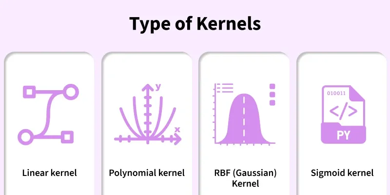 Types
TypesStepwise implementation of different SVM Kernels:
Step 1: Import Modules
Importing required modules.
- SVC from sklearn.svm to build SVM models
- make_classification to generate sample data
- numpy for numerical processing
- matplotlib.pyplot for visualization
Python
from sklearn import svm
from sklearn.datasets import make_classification
import matplotlib.pyplot as plt
import numpy as np
Step 2: Generate Synthetic Dataset
Creating a 2-feature dataset so decision boundaries can be visualized easily.
Python
X, y = make_classification(
    n_samples=300,
    n_features=2,
    n_redundant=0,
    n_informative=2,
    random_state=42
)
Step 3: Helper Function to Plot Decision Boundaries
This function creates a grid, predicts labels across the grid and draws classification regions.
Python
def plot_decision_boundary(model, X, y, title):
    x_min, x_max = X[:, 0].min() - 1, X[:, 0].max() + 1
    y_min, y_max = X[:, 1].min() - 1, X[:, 1].max() + 1

    xx, yy = np.meshgrid(
        np.linspace(x_min, x_max, 400),
        np.linspace(y_min, y_max, 400)
    )

    Z = model.predict(np.c_[xx.ravel(), yy.ravel()])
    Z = Z.reshape(xx.shape)

    plt.figure()
    plt.contourf(xx, yy, Z, alpha=0.3)
    plt.scatter(X[:, 0], X[:, 1], c=y)
    plt.title(title)
    plt.xlabel("Feature 1")
    plt.ylabel("Feature 2")
    plt.show()
Step 4: Train SVM with Linear Kernel
Linear kernel draws a straight line between classes.
Python
model_linear = svm.SVC(kernel='linear')
model_linear.fit(X, y)
plot_decision_boundary(model_linear, X, y, "SVM with Linear Kernel")
Output:
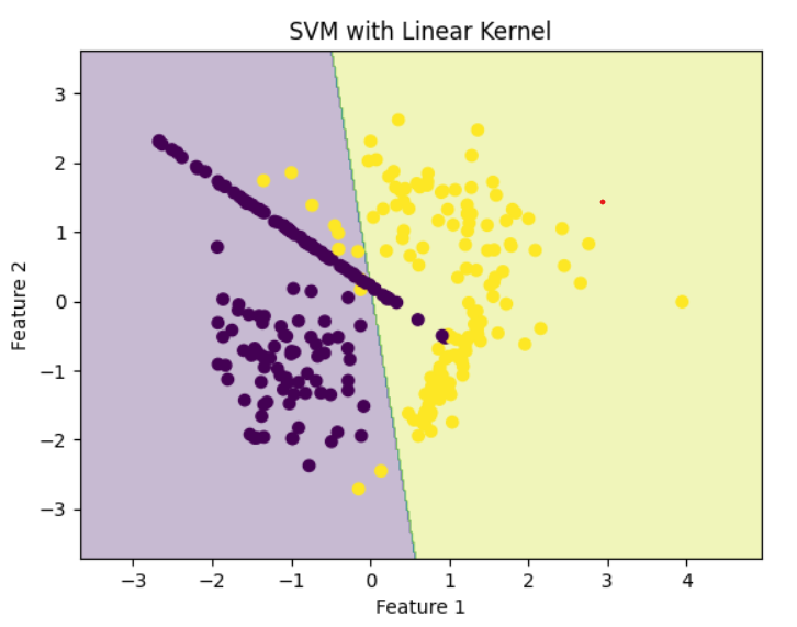 Linear Kernel
Step 5: Train SVM with Polynomial Kernel
Polynomial kernel generates curved, non-linear separation.
Python
model_poly = svm.SVC(kernel='poly', degree=3)
model_poly.fit(X, y)
plot_decision_boundary(model_poly, X, y, "SVM with Polynomial Kernel")
Output:
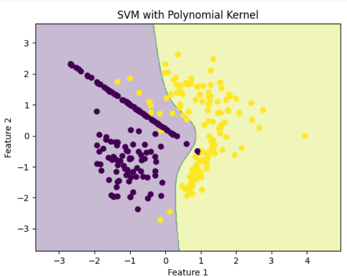 Polynomial Kernel
Step 6: Train SVM with RBF (Gaussian) Kernel
RBF kernel maps data to higher dimensions and creates smooth, complex surfaces.
Python
model_rbf = svm.SVC(kernel='rbf')
model_rbf.fit(X, y)
plot_decision_boundary(model_rbf, X, y, "SVM with RBF Kernel")
Output:
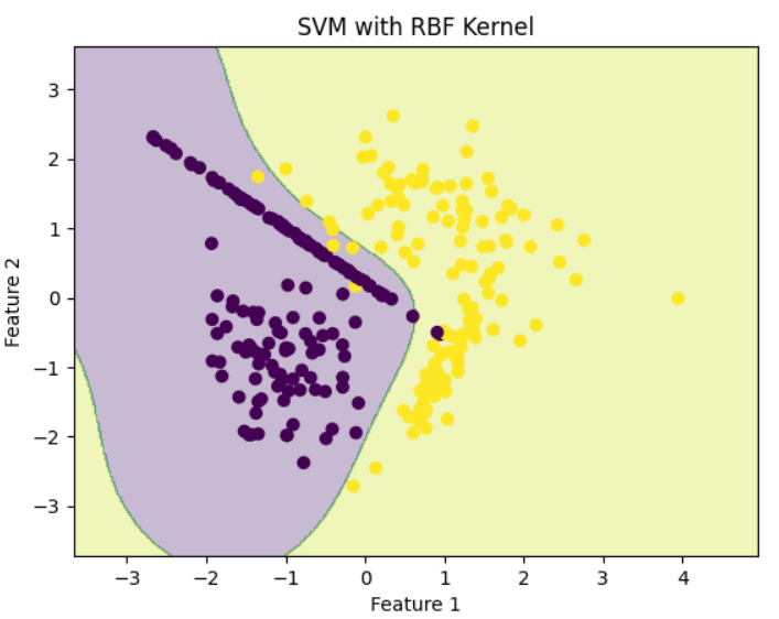 RBF Kernel
Step 7: Train SVM with Sigmoid Kernel
Sigmoid behaves similarly to neural network activation functions.
Python
model_sigmoid = svm.SVC(kernel='sigmoid')
model_sigmoid.fit(X, y)
plot_decision_boundary(model_sigmoid, X, y, "SVM with Sigmoid Kernel")
Output:
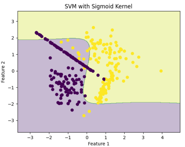 Sigmoid Kernel
Explore
Machine Learning Basics
Python for Machine Learning
Feature Engineering
Supervised Learning
Unsupervised Learning
Model Evaluation and Tuning
Advanced Techniques
Machine Learning Practice