Topos

Previously: Subobject Classifier.

In category theory, objects are devoid of internal structure. We’ve seen however that in certain categories we can define relationships between objects that mimic the set-theoretic idea of one set being the subset of another. We do this using the subobject classifier.

We would like to define a subobject classifier in the category of presheaves, so we could easily characterize subfunctors of a given presheaf. This will help us work with sieves, which are subfunctors of the hom-functor $C(-, a)$ ; and coverages, which are special kinds of sieves.

Recall that a presheaf $S$ is a subfunctor of another presheaf $P \colon C^{op} \to Set$ if it satisfies two conditions.

For every object $a$ , we have a set inclusion: $S a \subseteq P a$ ,
For every morphism $f \colon c \to a$ , the function $S f \colon S a \to S c$ is a restriction of the function $P f \colon P a \to P c$ . In other words, $P f$ and $S f$ must agree on the subset $S a$ .

As category theory goes, this is a very low-level definition. We need something more abstract: We need to construct a subobject classifier in the category of presheaves. Recall that a subobject classifier is defined by the following pullback diagram:

This time, however, the objects are presheaves and the arrows are natural transformations.

To begin with we have to define a terminal presheaf, $1 \colon C^{op} \to Set$ that satisfies the condition that, for any presheaf $P$ , there is a unique natural transformation $! \colon P \to 1$ . This will work if every component $!_a \colon P a \to 1 a$ of this natural transformation is unique, which is true if we choose $1 a$ to be the terminal singleton set $\{ * \}$ . Thus the terminal presheaf maps all objects to the terminal set, and all morphisms to the identity on $\{ * \}$ .

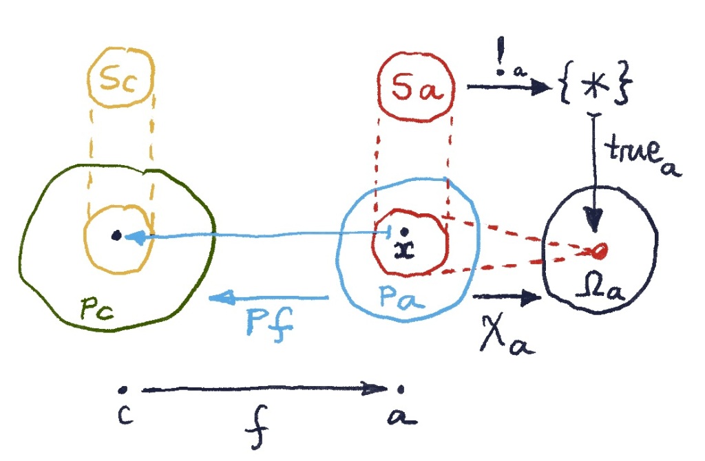
Next, let’s instantiate the subobject classifier diagram at a particular object $a$ .

Here, the component $true_a$ picks a special “True” element in the set $\Omega_a$ . If the presheaf $S$ is a subfunctor of $P$ , the set $S a$ is a subset of $P a$ . The function $\chi_a$ must therefore map the whole subset $S a$ to “True”. This is consistent with our definition of the subobject classifier for sets.

The second condition in the definition of a subfunctor is more interesting. It involves the mapping of morphisms.

The restriction condition

We have to consider all morphisms converging on our object of interest $a$ . For instance, lets take $f \colon c \to a$ . The presheaf $P$ lifts it to a function $P f \colon P a \to P c$ . If $S$ is a subfunctor of $P$ , $S f$ is a restriction of $P f$ .

Specifically the restriction condition tells us that, if we pick an element $x \in S a$ , then both $P f$ and $S f$ will map it to the same element of $S c$ . In fact, when defining a subobject, we only care if the embedding of $S c$ in $P c$ is injective (monomorphic). It’s okay if it permutes the elements of $S c$ . So it’s enough that, for all $x \in S a$ , the following condition is satisfied:

$(P f) x \in S c$

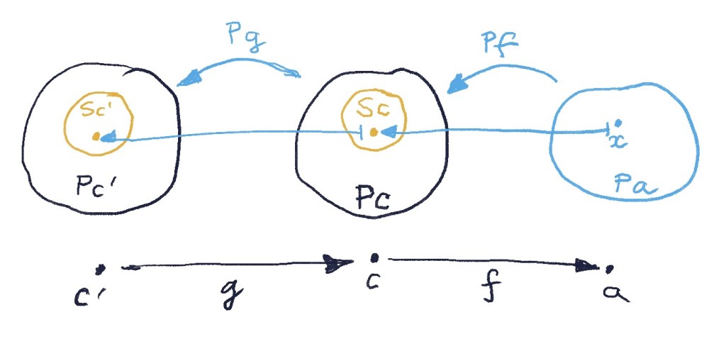
Now consider an arbitrary $x \in P a$ (not necessarily an element of $S a$ ). We can gather all arrows $f$ converging on $a$ for which the subset-mapping condition is satisfied:

$(P f) x \in S c$

If $S$ is a subfunctor of $P$ , these arrows form a sieve on $a$ , as any composition $f \circ g$ also satisfies the subset-mapping condition:

Moreover, if $x$ is in fact an element of $S a$ , this sieve is the maximal sieve. A maximal sieve on $a$ is a collection of all arrows converging on $a$ .

We can now define a function $\chi_a$ that assigns to each $x \in P a$ the sieve of arrows that satisfy the subset-mapping condition.

$\chi_a x = \{f \colon c \to a \, | \, (P f) x \in S c\}$

The function $\chi_a$ has the property that, if $x$ is an element of $S a$ , the result is the maximal sieve on $a$ .

It makes sense then to define $\Omega_a$ as a set of sieves on $a$ , and “True” as the maximal sieve on $a$ . (Thus $\Omega_a$ is a set whose elements are sets.)

The mapping $\Omega \colon a \to \Omega_a$ can be made into a presheaf by defining its action on morphisms. The lifting of $f \colon c \to a$ takes a sieve $s_a \in \Omega_a$ to a sieve $s'_{c} \in \Omega c$ , defined as a set of arrows $h \colon c' \to c$ , such that $f \circ h \in s_a$ .

Notice that the resulting sieve $s_c'$ is maximal if and only if $f \in \Omega_a$ . (Hint: If a sieve is maximal, then it contains identity.)

It can be shown that the the functions $\chi_a$ combine to form a natural transformation $\chi \colon P \to \Omega$ .

What remains to be shown is that this $\chi$ is a unique such natural transformation that completes the pullback:

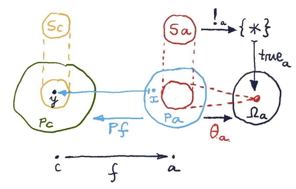
To show that, let’s assume that there is another natural transformation $\theta \colon P \to \Omega$ making this diagram into a pullback. Let’s redraw the subfunctor condition for arrows, replacing $\chi$ with $\theta$ :

Let’s pick an $x \in P a$ and call $y = (P f) x$ . We’ll follow a set of equivalences.

The pullback condition:

tells us that $y \in S c$ is equivalent to $\theta_c y = true_c$ . In other words:

$\theta_c ((P f) x) = true_c$

Using naturality of $\theta$ :

we can rewrite it as:

$(\Omega f) (\theta_a x) = true_c$ .

Both sides of this equation are sieves. By definition, the lifting of $f$ , $\Omega f$ , acting on $\theta_a x$ is a sieve defined by the following set of arrows:

$(\Omega f) (\theta_a x) = \{ h \colon c' \to c \, | \, f \circ h \in \theta_a x \}$

Since $true_c$ is a maximal sieve, it must be that $f \in \theta_a x$ .

We have shown that the condition $(P f) x \in S c$ is equivalent to $f \in \theta_a x$ . But the first condition is exactly the one we used to define $\chi_a x$ . Therefore $\chi$ is the only function that makes the subobject classifier diagram into a pullback.

Subfunctor classifier

The subobject classifier in the category of presheaves is thus a presheaf $\Omega$ that maps objects to sieves, together with the natural transformation $true \colon 1 \to \Omega$ that picks maximal sieves.

Every natural transformation $\chi \colon P \to \Omega$ defines a subfunctor of the presheaf $P$ . The components of this natural transformation serve as characteristic functions for the sets $P a$ . A given element $x$ is in the subset $S a$ iff $\chi_a$ maps it to the maximal sieve on $a$ .

But there’s not one but many different ways of failing the subset test. They are given by non-maximal sieves. We may think of them as satisfying the Anna Karenina principle, “All happy families are alike; each unhappy family is unhappy in its own way.”

Why sieves? Because once an element of a set $P a$ is mapped by $P f$ to an element of a subset $S c$ , it will continue to be mapped into consecutive subsets $S c'$ , etc. The network of “happy” morphisms keeps growing outward. By contrast, the “unhappy” elements of $x \in P a$ have at least one morphism $f \colon c \to a$ , whose lifting maps it outside the subset $S c$ . That’s the morphism that’s absent from the non-maximal sieve $\chi_a$ . Finally, naturality of $\chi$ ensures that subset conditions propagate coherently from object to object.

Next: Fibrations and Cofibrations.

Proviously Sieves and Sheaves.

We have seen how topology can be defined by working with sets of continuous functions over coverages. Categorically speaking, a coverage is a special case of a sieve, which is defined as a subfunctor of the hom-functor $C(-, a)$ .

We’d like to characterize the relationship between a functor and its subfunctor by looking at them as objects in the category of presheaves. For that we need to introduce the idea of a subobject.

We’ll start by defining subobjects in the category of sets in a way that avoids talking about elements. Here we have two options.

The first one uses a characteristic function. It’s a predicate that answers the question: Is some element $x$ a member of a given subset or not? Notice that any Boolean-valued function uniquely defines a subset of its domain, so we don’t really need to talk about elements, just a function.

But we still have to define a Boolean set. Let’s call this set $\Omega$ , and designate one of its element as “True.” Selecting “True” can be done by defining a function $true \colon 1 \to \Omega$ , where $1$ is the terminal object (here, a singleton set). In principle we should insist that $\Omega$ contains two elements, “True” and “False,” but that would make it more difficult to generalize.

The second way to define a subset $S \subseteq P$ is to provide an injective function $m \colon S \rightarrowtail P$ that embeds $S$ in $P$ . Injectivity guarantees that no two elements are mapped to the same element. The image of $m$ then defines the subset of $P$ . In a general category, injective functions are replaced by monics (monomorphisms).

Notice that there can be many injections that define the same subset. It’s okay for them to permute the image of $m$ as long as it covers exactly the same subset of $P$ . (These injections form an equivalence class.)

The fact that the two definitions coincide can be summarized by one commuting diagram. In the category of sets, given a characteristic function $\chi$ , the subset $S$ and the monic $m$ are uniquely (up to isomorphism) defined as a pullback of this diagram.

We can now turn the tables and use this diagram to define the object $\Omega$ called the subobject classifier, together with the monic $true \colon 1 \rightarrowtail \Omega$ . We do it by means of a universal construction. We postulate that: For every monic $S \rightarrowtail P$ between two arbitrary objects there exist a unique arrow $\chi \colon P \to \Omega$ such that the above diagram constitutes a pullback.

This is a slightly unusual definition. Normally we think of a pullback as defining the northwest part of the diagram given its southeast part. Here, we are solving a sudoku puzzle, trying to fill the southeast part to uniquely complete a pullback diagram.

Let’s see how this works for sets. To construct a pullback (a.k.a., a fibered product $P \times_{\Omega} 1$ ) we first create a set of pairs $(x, *)$ where $x \in P$ and $* \in 1$ (the only element of the singleton set). But not all $x$ ‘s are acceptable, because we have a pullback condition, which says that $\chi x = \text{True}$ , where $\text{True}$ is the element of $\Omega$ pointed to by $true$ . This tells us that $S$ is isomorphic to the subset of $P$ for which $\chi$ is $\text{True}$ .

The question is: What happens to the other elements of $P$ ? They cannot be mapped to $\text{True}$ , so $\Omega$ must contain at least one more element (in case $m$ is not an isomorphism). Can it contain more?

This is where the universal construction comes into play. Any monic $m$ (here, an injective function) must uniquely determine a $\chi$ that completes the pullback. In particular, we can pick $S$ to be a singleton set and $P$ to be a two-element set. We see that if $\Omega$ contained only $\text{True}$ and nothing else, no $\chi$ would complete the pullback. And if $\Omega$ contained more than two elements, there would be not one but at least two such $\chi$ ‘s. So, by the Goldilock principle, $\Omega$ must have exactly two elements.

We’ll see later that this is not necessarily true in a more general category.

Next: Subfunctor Classifier.

Bartosz Milewski's Programming Cafe

Subfunctor Classifier

The restriction condition

Subfunctor classifier

Subobject Classifier

Top Posts

License

Blogroll

Follow Me

Archives