math | Bartosz Milewski's Programming Cafe

July 26, 2025

(Weak) Factorization Systems

Posted by Bartosz Milewski under Homotopy, Topology | Tags: Homotopy, math, Topology |
Leave a Comment

Previously (Weak) Homotopy Equivalences.

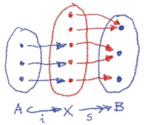
An average function between sets, $f \colon A \to B$ is neither surjective nor injective. We can however isolate the two “failure modes” if we insert a third set $X$ in between. We can, for instance, pick this set to be the subset of $B$ that is the image of $A$ under $f$ . We then define $s \colon A \twoheadrightarrow X$ to be the surjective part of $f$ . This way $s$ deals just with all the non-injectivity of $f$ . We can then follow $s$ with an injective function $i \colon X \hookrightarrow B$ . We get the (Surj, Inj) factorization of an arbitrary function into a surjection followed by an injection:

$f = i \circ s$

This factorization is unique up to unique isomorphism.

Notice also that both surjections and injections are closed under composition and that every isomorphism is simultaneously a surjection and an injection.

In category theory we generalize this idea to define abstract factorization systems.

A (strict) factorization system specifies two classes of morphisms $L$ and $R$ , satisfying conditions loosely analogous to the (Surj, Inj) factorization:

Each class is closed under composition and contains all isomorphisms.
Every morphism can be factorized, $f = r \circ l$ , with $l \in L$ and $r \in R$
The factorization is functorial.

The last condition requires some explanation. We can look at factorization as a functor between two categories.

The source category is the arrow category of $C$ . Its objects are arrows or, more precisely, triples $(a, b, f \colon a \to b)$ . A morphism from $(a, b, f)$ to $(a', b', f')$ is a pair of arrows $(u \colon a \to a', v \colon b \to b')$ that make the following square commute:

The target category is the category of factorizations. Its objects are factorizations, or pairs of composable arrows $(l, r)$ :

$a \xrightarrow{l} x \xrightarrow{r} b$

taken from the two classes $(L, R)$ . Morphisms are triples of arrows $(u, w, v)$ that make the following diagram commute:

The functor in question maps an arrow $(a, b, f)$ to its factorization, $a \xrightarrow{l} x \xrightarrow{r} b$ , with $f = r \circ l$ . Its action on a morphism $(u, v)$ is the commuting diagram above. For functoriality, we need the arrow $w$ to be determined uniquely.

Notice that we can redraw the last diagram in such a way that $w$ crosses it diagonally.

In other words, morphisms in $L$ have the (strict) left lifting property with respect to morphisms in $R$ .

Interesting things start happening when we relax the strictness property and allow $w$ not to be unique. We can no longer talk about functoriality of factorization. Instead we lean on the (weak) lifting property.

To illustrate this, let’s reverse the roles of surjections and injections in our factorization of functions. Indeed, every function can be factored into an injection followed by a surjection. Such (Inj, Surj) factorization is not unique. (It also requires the use of the Axiom of Choice.)

A weak factorization system consists, as before, of two classes of morphisms $(L, R)$ that allow for factoriziation of an arbitrary morphism $f = l \circ r$ . This time, however, we postulate that $L$ is precisely the class of morphisms with a left lifting property against every morphism in $R$ ; and vice versa for $R$ and the right lifting property.

At this point you may recall the lifting property we discussed earlier between fibrations and cofibrations. In particular, a cofibration satisfies the homotopy extension property.

Interestingly, there is a connection between fibrations and surjections, and cofibrations and injections.

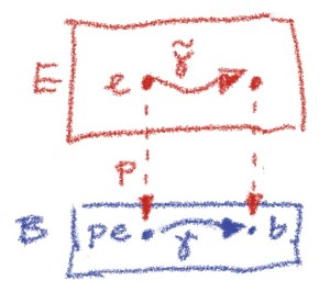
First, we’ll show that a fibration $p \colon E \to B$ is a surjection as long as $E$ is non empty and $B$ is path connected.

Here’s the proof: If $p$ were not surjective then there would be a point $b \in B$ that is not in the image of $p$ . Since $E$ is not empty, there exists a point $e \in E$ . Take any path $\gamma$ in $B$ connecting $p \, e$ to $b$ . Since $p$ is a fibration, we can lift this path to $\tilde{\gamma}$ in $E$ . Since $p$ projects the endpoint of $\tilde{\gamma}$ to $b$ , we have reached a contradiction. Therefore $p$ must be a surjection. $\blacksquare$

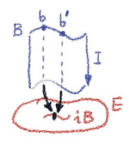
The proof that every cofibration is injective is a bit more involved. It uses a very handy notion of a mapping cylinder. We can visualize a function $i \colon B \to E$ between two spaces as a bunch of wires. Each wire connects a point $b \in B$ to the corresponding point $i \, b \in E$ . A mapping cylinder $M_i$ is a topological space that formalizes this picture.

We start with pairs $(b, t) \in B \times I$ , where $I$ is the unit segment, which we use to parameterize the length of each wire. Then we add the target $E$ to our cylinder, and plug the end $(b, 1)$ of each wire to its “socket” $i \, b \in E$ .

Formally, the mapping cylinder $M_i$ is a quotient space of the disjoint union $(B \times I) \bigsqcup E$ , identifying each $(b, 1)$ with $i \, b$ .

Notice that, if $i$ is not injective, there will be some merging of multiple wires right when they hit $E$ , but not earlier–the fact that will become relevant later.

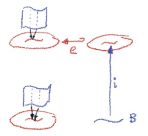
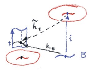
Now let’s use the cofibration property of $i$ . We replace the big space $X$ with the cylinder $M_i$ . The arrow $e$ is the inclusion $e \colon E \hookrightarrow M_i$ . Notice that $e$ will be identified with the starting point of the homotopy $\tilde h_0$ that we’re constructing.

First we define the homotopy $h \colon B \times I \to M_i$ . For every $t \in I$ , we write $h_t \colon B \to M_i$ .

At $t = 0$ , $h_0\, b$ is the point in $M_i$ that sits on the seam between $B \times I$ and $E$ . In our quotient space, it corresponding to $i \, b$ .

For $t > 0$ we define $h_t \, b = \{(b, 1-t)\}$ . It reverses the direction of wires in the cylinder $M_i$ . (We use curly braces to embed the pair $(b, 1-t) \in B \times I$ into the quotient $M_i$ .)

The function $h$ is continuous, therefore a homotopy. (It may still merge multiple points into one, if $i$ is not injective.)

Cofibration condition states that any homotopy $h \colon B \times I \to M_i$ can be lifted to $\tilde h \colon E \times I \to M_i$ , such that $h (b, t) =\tilde h (i \, b, t)$ . The latter condition can be written as:

$h_t = \tilde h_t \circ i$

In our case, $\tilde h_0$ will shrink the whole of $E$ down to $i \, B$ before embedding it in $M_i$ .

Then, for any $t > 0$ , $\tilde h_t$ will shrink $E$ down to $B$ , embed it in $B \times I$ at $1 - t$ , and inject it into $M_i$ .

Notice that, for any fixed $t > 0$ , our $h_t$ is injective ( $h$ could only do the merging of wires at $t = 0$ , where the identification happens). But the lifting condition tells us that $h_t = \tilde h_t \circ i$ . Therefore $i$ must also be injective. $\blacksquare$

We have shown that fibrations between (path-connected, non-empty) topological spaces are surjective, and that cofibrations are injective.

Corresponding to the weak (Inj, Surj) factorization system in Set, we can build a weak (Cofib, Fib) factorization system in Top (the category of topological spaces). Indeed, under some conditions, every continuous function can be factored into a cofibration followed by a fibration.

We’ve seen earlier that cofibrations have the left lifting property with respect to fibrations, and vice versa. So (Cofib, Fib) is indeed an example of a weak factorization system. We’ll see later that weak factorization systems form the basis of Quillen model categories.

Next: Models of (Dependent) Type Theory.

June 20, 2025

(Weak) Homotopy Equivalences

Posted by Bartosz Milewski under Category Theory, Homotopy, Homotopy Type Theory, Topology | Tags: Category Theory, Homotopy, math, Topology |
Leave a Comment

Previously: Fibrations and Cofibrations.

In topology, we say that two shapes are the same if there is a homeomorphism– an invertible continuous map– between them. Continuity means that nothing is broken and nothing is glued together. This is how we can turn a coffe cup into a torus. A homeomorphism, however, won’t let us shrink a torus to a circle. So if we are only interested in how many holes the shapes have, we have to relax our notion of equivalence.

Let’s go back to the definition of homeomorphism. It is defined as a pair of continuous functions between two topological spaces, $f \colon X \to Y$ and $g \colon Y \to X$ , such that their compositions are identity maps, $f \circ g = id_Y$ and $g \circ f = id_X$ , respectively.

If we want to allow for extreme shrinkage, as with a (solid) torus shrinking down to a circle, we have to relax the identity conditions.

A homotopy equivalence is a pair of continuous functions, but their compositions don’t have to be equal to identities. It’s enough that they are homotopic to identities. In other words, it’s possible to create an animation that transforms one to another.

Take the example of a line $\mathbb R$ and a point. The point is a trivial topological space where only the whole space (here, the singleton $\{*\}$ ) and the empty set are open. $\mathbb R$ and $\{*\}$ are obviously not homeomorphic, but they don’t have any holes, so they should be homotopy equivalent.

Indeed, let’s construct the equivalence as a pair of constant functions: $f \colon x \mapsto *$ and $g \colon * \mapsto 0$ (the origin of $\mathbb R$ ). Both are continuous: The pre-image $f^{-1} \{ * \}$ is the whole real line, which is open. The pre-image $g^{-1}$ of any open set in $\mathbb R$ is $\{*\}$ , which is also open.

The composition $f \circ g \colon * \mapsto *$ is equal to the identity on $\{*\}$ , so it’s automatically homotopic to it. The interesting part is the composition $g \circ f \colon x \mapsto 0$ , which is emphatically not equal to identity on $\mathbb R$ . We can however construct a homotpy between the identity and it. It’s a function that interpolates between them:

$h \colon \mathbb R \times I \to \mathbb R$

$h (x, 0) = id_{\mathbb R} x = x$

$h(x, 1) = (g \circ f) x = 0$

( $I$ is the unit interval $[0, 1]$ .) Such a function exists:

$h (x, t) = (1 - t) \,x$

When a space is homotopy equivalent to a point, we say that it’s contractible. Thus $\mathbb R$ is contractible. Similarly, n-dimensional spaces, $\mathbb R^n$ , as well as n-dimensional balls are all contractible. A circle, however, is not contractible, because it has a hole.

Another way of looking for holes in spaces is by trying to shrink loops. If there is a hole inside a loop, it cannot be continuously shrunk to a point. Imagine a loop going around a circle. There is no way you can “unwind” it without breaking something. In fact, you can have loops that wind n times around a circle. They can’t be homotopied into each other if their winding numbers are different.

In general, paths in a topological space $X$ , i.e. continuous mappings $\gamma \colon I \to X$ , naturally split into equivalence classes with respect to homotopy. Two paths, $\gamma$ and $\gamma'$ , sharing the same endpoints are in the same class if there is a homotopy between them:

$h \colon I \times I \to X$

$h (0, t) = \gamma t$

$h (1, t) = \gamma' t$

Moreover, two paths can be composed, as long as the endpoint of one coincides with the start point of the other (after performing appropriate reparametrizations).

There is a unit of such composition, a constant path; and every path has its inverse, a path that traces the original but goes in the opposite direction.

It’s easy to see that path composition induces a groupoid structure on the set of equivalence classes of paths. A groupoid is a category in which every morphism (here, path) is invertible. This particular groupoid is called the fundamental groupoid of the topological space $X$ .

If we pick a base point $x_0$ in $X$ , the paths that start and end at this point form closed loops. These loops then form a fundamental group $\pi_1(X, x_0)$ .

Notice that, as long as there is a path $\gamma$ from $x_0$ to $x_1$ , the fundamental groups at both points are isomorphic. This is because every loop $l$ at $x_1$ induces a loop at $x_0$ given by the concatenation $l' = \gamma^{-1} \circ l \circ \gamma$ .

So there is essentially a single fundamental group for the whole space, as long as $X$ is path-connected, i.e., it doesn’t split into multiple disconnected chunks.

Going back to our example of a circle, its fundamental group is the group of integers $\mathbb Z$ with addition. All loops that wind n-times around the circle in one direction correspond to the integer n.

Negative integers correspond to loops winding in the opposite direction. If you follow an n-loop with an m-loop, you get an (m+n)-loop. Zero corresponds to loops that can be shrunk to a point.

To tie these two notions of hole-counting together, it can be shown that two spaces that are homotopy equivalent also have the same fundamental groups. This makes sense, since equivalent spaces have the same holes.

Not only that, they also have the same higher homotopy groups (as long as both are path-connected).

We define the n-th homotopy group by replacing simple loops (which are homotopic to a circle, or a 1-dimensional sphere) with n-dimensional spheres. Attempts at shrinking those may detect higher-dimensional holes.

For instance, imagine an Earth-like ball with it’s inner core scooped out. Any 1-loop inside its bulk can be shrunk to a point (it will glide off the core). But a 2-sphere that envelops the core cannot be shrunk.

In fact such a 2-sphere can be wrapped around the core an arbitrary number of times. In math notation, we say:

$\pi_2 (B^3 \setminus \{ 0 \}) = \mathbb Z$

Corresponding to these higher homotopy groups there is also a higher homotopy groupoid, in which there are invertible paths, surfaces between paths, volumes between surfaces, etc. Taken together, these form an infinity groupoid. It is exactly the inspiration behind the infinity groupoid in homotopy type theory, HoTT.

Spaces that are homotopy equivalent have the same homotopy groups, but the converse is not true. There are spaces that are not homotopy equivalent even though they have the same homotopy groups. This is why a weaker version of equivalence was introduced.

A map between topological spaces is called a weak homotopy equivalence if it induces isomorphisms between all homotopy groups.

There is a subtle difference between strong and weak equivalences. Strong equivalence can be broken by a local anomaly, like in the following example: Take $X = \{0, 1, 2, ... \}$ , the set of natural numbers in which every number is considered an open set. Take $Y = \{ 0 \} \cup \{ 1, \frac{1}{2}, \frac{1}{3}, ... \}$ with the topology inherited from the real line.

The singleton set $\{ 0 \}$ in $Y$ is the obstacle to constructing a homeomorphism or a homotopy equivalence between $X$ and $Y$ . That’s because it is not open (there is no open set in $\mathbb R$ that contains it and nothing else). However, it’s impossible to have a non-trivial loop that would contain it, so $X$ and $Y$ are weakly equivalent.

Grothendieck conjectured that the infinity groupoid captures all information about a topological space up to weak homotopy equivalence.

Weak equivalences, together with fibrations and cofibrations, form the foundation of weak factorization systems and Quillen model categories.
Next: (Weak) Factorization Systems.

April 21, 2025

Subfunctor Classifier

Posted by Bartosz Milewski under Category Theory, Topology, Topos | Tags: Category Theory, math, Topology, Topos |
Leave a Comment

Previously: Subobject Classifier.

In category theory, objects are devoid of internal structure. We’ve seen however that in certain categories we can define relationships between objects that mimic the set-theoretic idea of one set being the subset of another. We do this using the subobject classifier.

We would like to define a subobject classifier in the category of presheaves, so we could easily characterize subfunctors of a given presheaf. This will help us work with sieves, which are subfunctors of the hom-functor $C(-, a)$ ; and coverages, which are special kinds of sieves.

Recall that a presheaf $S$ is a subfunctor of another presheaf $P \colon C^{op} \to Set$ if it satisfies two conditions.

For every object $a$ , we have a set inclusion: $S a \subseteq P a$ ,
For every morphism $f \colon c \to a$ , the function $S f \colon S a \to S c$ is a restriction of the function $P f \colon P a \to P c$ . In other words, $P f$ and $S f$ must agree on the subset $S a$ .

As category theory goes, this is a very low-level definition. We need something more abstract: We need to construct a subobject classifier in the category of presheaves. Recall that a subobject classifier is defined by the following pullback diagram:

This time, however, the objects are presheaves and the arrows are natural transformations.

To begin with we have to define a terminal presheaf, $1 \colon C^{op} \to Set$ that satisfies the condition that, for any presheaf $P$ , there is a unique natural transformation $! \colon P \to 1$ . This will work if every component $!_a \colon P a \to 1 a$ of this natural transformation is unique, which is true if we choose $1 a$ to be the terminal singleton set $\{ * \}$ . Thus the terminal presheaf maps all objects to the terminal set, and all morphisms to the identity on $\{ * \}$ .

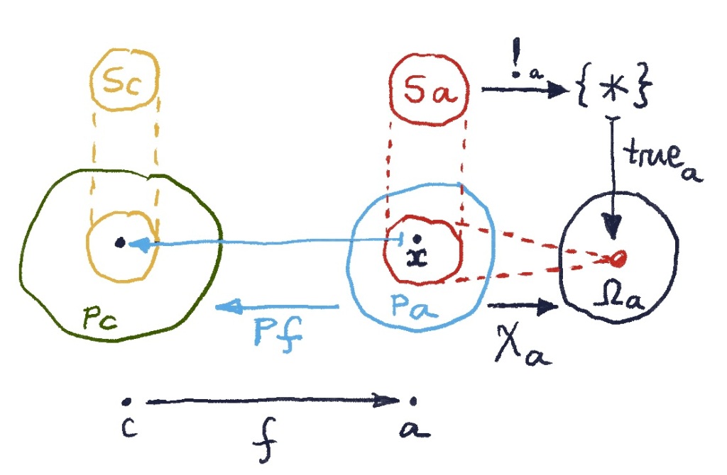
Next, let’s instantiate the subobject classifier diagram at a particular object $a$ .

Here, the component $true_a$ picks a special “True” element in the set $\Omega_a$ . If the presheaf $S$ is a subfunctor of $P$ , the set $S a$ is a subset of $P a$ . The function $\chi_a$ must therefore map the whole subset $S a$ to “True”. This is consistent with our definition of the subobject classifier for sets.

The second condition in the definition of a subfunctor is more interesting. It involves the mapping of morphisms.

The restriction condition

We have to consider all morphisms converging on our object of interest $a$ . For instance, lets take $f \colon c \to a$ . The presheaf $P$ lifts it to a function $P f \colon P a \to P c$ . If $S$ is a subfunctor of $P$ , $S f$ is a restriction of $P f$ .

Specifically the restriction condition tells us that, if we pick an element $x \in S a$ , then both $P f$ and $S f$ will map it to the same element of $S c$ . In fact, when defining a subobject, we only care if the embedding of $S c$ in $P c$ is injective (monomorphic). It’s okay if it permutes the elements of $S c$ . So it’s enough that, for all $x \in S a$ , the following condition is satisfied:

$(P f) x \in S c$

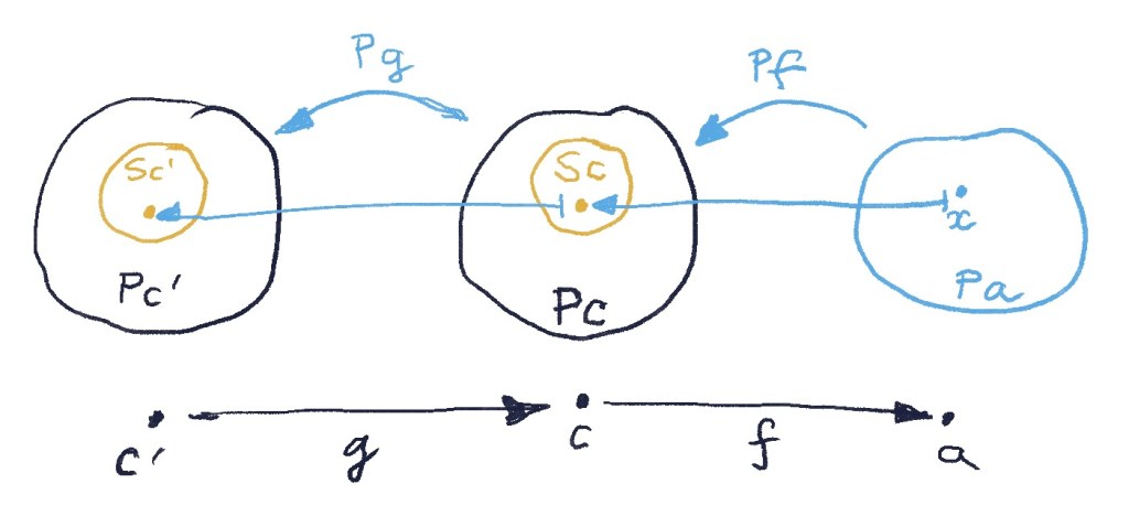
Now consider an arbitrary $x \in P a$ (not necessarily an element of $S a$ ). We can gather all arrows $f$ converging on $a$ for which the subset-mapping condition is satisfied:

$(P f) x \in S c$

If $S$ is a subfunctor of $P$ , these arrows form a sieve on $a$ , as any composition $f \circ g$ also satisfies the subset-mapping condition:

Moreover, if $x$ is in fact an element of $S a$ , this sieve is the maximal sieve. A maximal sieve on $a$ is a collection of all arrows converging on $a$ .

We can now define a function $\chi_a$ that assigns to each $x \in P a$ the sieve of arrows that satisfy the subset-mapping condition.

$\chi_a x = \{f \colon c \to a \, | \, (P f) x \in S c\}$

The function $\chi_a$ has the property that, if $x$ is an element of $S a$ , the result is the maximal sieve on $a$ .

It makes sense then to define $\Omega_a$ as a set of sieves on $a$ , and “True” as the maximal sieve on $a$ . (Thus $\Omega_a$ is a set whose elements are sets.)

The mapping $\Omega \colon a \to \Omega_a$ can be made into a presheaf by defining its action on morphisms. The lifting of $f \colon c \to a$ takes a sieve $s_a \in \Omega_a$ to a sieve $s'_{c} \in \Omega c$ , defined as a set of arrows $h \colon c' \to c$ , such that $f \circ h \in s_a$ .

Notice that the resulting sieve $s_c'$ is maximal if and only if $f \in \Omega_a$ . (Hint: If a sieve is maximal, then it contains identity.)

It can be shown that the the functions $\chi_a$ combine to form a natural transformation $\chi \colon P \to \Omega$ .

What remains to be shown is that this $\chi$ is a unique such natural transformation that completes the pullback:

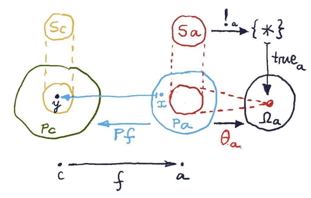
To show that, let’s assume that there is another natural transformation $\theta \colon P \to \Omega$ making this diagram into a pullback. Let’s redraw the subfunctor condition for arrows, replacing $\chi$ with $\theta$ :

Let’s pick an $x \in P a$ and call $y = (P f) x$ . We’ll follow a set of equivalences.

The pullback condition:

tells us that $y \in S c$ is equivalent to $\theta_c y = true_c$ . In other words:

$\theta_c ((P f) x) = true_c$

Using naturality of $\theta$ :

we can rewrite it as:

$(\Omega f) (\theta_a x) = true_c$ .

Both sides of this equation are sieves. By definition, the lifting of $f$ , $\Omega f$ , acting on $\theta_a x$ is a sieve defined by the following set of arrows:

$(\Omega f) (\theta_a x) = \{ h \colon c' \to c \, | \, f \circ h \in \theta_a x \}$

Since $true_c$ is a maximal sieve, it must be that $f \in \theta_a x$ .

We have shown that the condition $(P f) x \in S c$ is equivalent to $f \in \theta_a x$ . But the first condition is exactly the one we used to define $\chi_a x$ . Therefore $\chi$ is the only function that makes the subobject classifier diagram into a pullback.

Subfunctor classifier

The subobject classifier in the category of presheaves is thus a presheaf $\Omega$ that maps objects to sieves, together with the natural transformation $true \colon 1 \to \Omega$ that picks maximal sieves.

Every natural transformation $\chi \colon P \to \Omega$ defines a subfunctor of the presheaf $P$ . The components of this natural transformation serve as characteristic functions for the sets $P a$ . A given element $x$ is in the subset $S a$ iff $\chi_a$ maps it to the maximal sieve on $a$ .

But there’s not one but many different ways of failing the subset test. They are given by non-maximal sieves. We may think of them as satisfying the Anna Karenina principle, “All happy families are alike; each unhappy family is unhappy in its own way.”

Why sieves? Because once an element of a set $P a$ is mapped by $P f$ to an element of a subset $S c$ , it will continue to be mapped into consecutive subsets $S c'$ , etc. The network of “happy” morphisms keeps growing outward. By contrast, the “unhappy” elements of $x \in P a$ have at least one morphism $f \colon c \to a$ , whose lifting maps it outside the subset $S c$ . That’s the morphism that’s absent from the non-maximal sieve $\chi_a$ . Finally, naturality of $\chi$ ensures that subset conditions propagate coherently from object to object.

Next: Fibrations and Cofibrations.

March 20, 2025

Subobject Classifier

Posted by Bartosz Milewski under Category Theory, Topology, Topos | Tags: Category Theory, math, Topology |
Leave a Comment

Proviously Sieves and Sheaves.

We have seen how topology can be defined by working with sets of continuous functions over coverages. Categorically speaking, a coverage is a special case of a sieve, which is defined as a subfunctor of the hom-functor $C(-, a)$ .

We’d like to characterize the relationship between a functor and its subfunctor by looking at them as objects in the category of presheaves. For that we need to introduce the idea of a subobject.

We’ll start by defining subobjects in the category of sets in a way that avoids talking about elements. Here we have two options.

The first one uses a characteristic function. It’s a predicate that answers the question: Is some element $x$ a member of a given subset or not? Notice that any Boolean-valued function uniquely defines a subset of its domain, so we don’t really need to talk about elements, just a function.

But we still have to define a Boolean set. Let’s call this set $\Omega$ , and designate one of its element as “True.” Selecting “True” can be done by defining a function $true \colon 1 \to \Omega$ , where $1$ is the terminal object (here, a singleton set). In principle we should insist that $\Omega$ contains two elements, “True” and “False,” but that would make it more difficult to generalize.

The second way to define a subset $S \subseteq P$ is to provide an injective function $m \colon S \rightarrowtail P$ that embeds $S$ in $P$ . Injectivity guarantees that no two elements are mapped to the same element. The image of $m$ then defines the subset of $P$ . In a general category, injective functions are replaced by monics (monomorphisms).

Notice that there can be many injections that define the same subset. It’s okay for them to permute the image of $m$ as long as it covers exactly the same subset of $P$ . (These injections form an equivalence class.)

The fact that the two definitions coincide can be summarized by one commuting diagram. In the category of sets, given a characteristic function $\chi$ , the subset $S$ and the monic $m$ are uniquely (up to isomorphism) defined as a pullback of this diagram.

We can now turn the tables and use this diagram to define the object $\Omega$ called the subobject classifier, together with the monic $true \colon 1 \rightarrowtail \Omega$ . We do it by means of a universal construction. We postulate that: For every monic $S \rightarrowtail P$ between two arbitrary objects there exist a unique arrow $\chi \colon P \to \Omega$ such that the above diagram constitutes a pullback.

This is a slightly unusual definition. Normally we think of a pullback as defining the northwest part of the diagram given its southeast part. Here, we are solving a sudoku puzzle, trying to fill the southeast part to uniquely complete a pullback diagram.

Let’s see how this works for sets. To construct a pullback (a.k.a., a fibered product $P \times_{\Omega} 1$ ) we first create a set of pairs $(x, *)$ where $x \in P$ and $* \in 1$ (the only element of the singleton set). But not all $x$ ‘s are acceptable, because we have a pullback condition, which says that $\chi x = \text{True}$ , where $\text{True}$ is the element of $\Omega$ pointed to by $true$ . This tells us that $S$ is isomorphic to the subset of $P$ for which $\chi$ is $\text{True}$ .

The question is: What happens to the other elements of $P$ ? They cannot be mapped to $\text{True}$ , so $\Omega$ must contain at least one more element (in case $m$ is not an isomorphism). Can it contain more?

This is where the universal construction comes into play. Any monic $m$ (here, an injective function) must uniquely determine a $\chi$ that completes the pullback. In particular, we can pick $S$ to be a singleton set and $P$ to be a two-element set. We see that if $\Omega$ contained only $\text{True}$ and nothing else, no $\chi$ would complete the pullback. And if $\Omega$ contained more than two elements, there would be not one but at least two such $\chi$ ‘s. So, by the Goldilock principle, $\Omega$ must have exactly two elements.

We’ll see later that this is not necessarily true in a more general category.

Next: Subfunctor Classifier.

November 16, 2024

Sieves and Sheaves

Posted by Bartosz Milewski under Category Theory, Topology | Tags: Category Theory, math, mathematics, Topology |
Leave a Comment

Previously: Covering Sieves.

We’ve seen an intuitive description of presheaves as virtual objects. We can use the same trick to visualize natural transformations.

A natural transformation can be drawn as a virtual arrow $\alpha$ between two virtual objects corresponding to two presheaves $S$ and $P$ . Indeed, for every $s_a \in S a$ , seen as an arrow $a \to S$ , we get an arrow $a \to P$ simply by composition $\alpha \circ s_a$ . Notice that we are thus defining the composition with $\alpha$ , because we are outside of the original category. A component $\alpha_a$ of a natural transformation is a mapping between two arrows.

Untitled Artwork

This composition must be associative and, indeed, associativity is guaranteed by the naturality condition. For any arrow $f \colon a \to b$ , consider a zigzag path from $a$ to $P$ given by $\alpha \circ s_b \circ f$ . The two ways of associating this composition give us $\alpha_a \circ S f = P f \circ \alpha_b$ .

Untitled Artwork

Let’s now recap our previous definitions: A cover of $u$ is a bunch of arrows converging on $u$ satisfying certain conditions. These conditions are defined in terms of a coverage. For every object $u$ we define a whole family of covers, and then combine them into one big collection that we call the coverage.

A sheaf is a presheaf that is compatible with a coverage. It means that for every cover $\{u_i\}$ , if we pick a compatible family of $x_i \in P u_i$ that agrees on all overlaps, then this uniquely determines the element (virtual arrow) $x \in P u$ .

Untitled Artwork

A covering sieve of $u$ is a presheaf that extends a cover $\{u_i\}$ . It assigns a singleton set to each $u_i$ and all its open subsets (that is objects that have arrows pointing to $u_i$ ); and an empty set otherwise. In particular, the sieve includes all the overlaps, like $u_i \cap u_j$ , even if they are not present in the original cover.

The key observation here is that a sieve can serve as a blueprint for, or a skeleton of, a compatible family $\{ x_i \}$ . Indeed, $S_u$ maps all objects either to singletons or to empty sets. In terms of virtual arrows, there is at most one arrow going to $S_u$ from any object. This is why a natural transformation from $S_u$ to any presheaf $P$ produces a family of arrows $x_i \in P u_i$ . It picks a single arrow from each of the hom-sets $u_i \to P$ .

Untitled Artwork

The sieve includes all intersections, and all diagrams involving those intersections necessarily commute. They commute because the category we’re working with is thin, and so is the category extended by adding the virtual object $S_u$ . Thus a family generated by a natural transformation $\alpha \in Nat (S_u, P)$ is automatically a compatible family. Therefore, if $P$ is a sheaf, it determines a unique element $x \in P u$ .

This lets us define a sheaf in terms of sieves, rather than coverages.

A presheaf $P$ is a sheaf if and only if, for every covering sieve $S_u$ of every $u$ , there is a one-to-one correspondence between the set of natural transformations $Nat (S_u, P)$ and the set $P u$ .

In terms of virtual arrows, this means that there is a one-to-one correspondence between arrows $\alpha \colon S_u \to P$ and $x \colon u \to P$ .

Untitled Artwork
Next: Subobject Classifier

October 31, 2024

Covering Sieves

Posted by Bartosz Milewski under Category Theory, Topology | Tags: Category Theory, math, mathematics, Topology |
[2] Comments

Previously: Sheaves as Virtual Objects.

In order to define a sheaf, we have to start with coverage. A coverage defines, for every object $u$ , a family of covers that satisfy the sub-coverage conditions. Granted, we can express coverage using objects and arrows, but it would be much nicer if we could use the language of functors and natural transformations.

Let’s start with the idea that, categorically, a cover of $u$ is a bunch of arrows converging on $u$ . Each arrow $p_i \colon u_i \to u$ is a member of the hom-set $\mathcal C (u_i, u)$ . Now consider the fact that $\mathcal C (-, u)$ is a presheaf, $\mathcal C^{op} \to \mathbf{Set}$ , and ask the question: Is a cover a “subfunctor” of $\mathcal C (-, u)$ ?

A subfunctor of a presheaf $P$ is defined as a functor $S$ such that, for each object $v$ , $S v$ is a subset of $P v$ and, for each arrow $f \colon v \to w$ , the function $S f \colon S w \to S v$ is a restriction of $P f$ .

Untitled Artwork

In general, a cover does not correspond to a subfunctor of the hom-functor. Let’s see why, and how we can fix it.

Let’s try to define $S$ , such that $S u_i$ is non-empty for any object $u_i$ that’s in the cover of $u$ , and empty otherwise. As a presheaf, we could represent it as a virtual object with arrows coming from all $\{ u_i \}$ ‘s.

Untitled Artwork

Now consider an object $v$ that is not in the cover, but it has an arrow $f \colon v \to u_k$ connecting it to some element $u_k$ of the cover. Functoriality requires the (virtual) composition $s_k \circ f$ to exist. Untitled Artwork

Thus $v$ must be included in the cover–if we want $S$ to be a functor.

In particular, if we are looking at a category of open sets with inclusions, this condition means that all (open) sub-sets of the covering sets must also be included in the cover. Such a “downward closed” family of sets is called a sieve.

Imagine sets in the cover as holes in a sieve. Smaller sets that can “pass through” these holes must also be parts of the sieve.

If you start with a cover, you can always extend it to a covering sieve by adding more arrows. It’s as if you started with a few black holes, and everything that could fall into them, would fall.

We have previously defined sheaves in terms of coverings. In the next installment we’ll see that they can equally well be defined using covering sieves.

Next Sieves and Sheaves.

October 24, 2024

Sheaves as Virtual Objects

Posted by Bartosz Milewski under Category Theory, Topology | Tags: Category Theory, math, mathematics, Topology |
1 Comment

Previously: Coverages and Sites

The definition of a sheaf is rather complex and involves several layers of abstraction. To help us navigate this maze we can use some useful intuitions. One such intuition is to view objects in our category as some kind of sets (in particular, open sets, when we talk about topology), and arrows as set inclusions. An arrow from $v$ to $u$ means that $v$ is a subset of $u$ .

A cover of $u$ is a family of arrows $\{ p_i \colon u_i \to u \}$ . A coverage assigns a collection of covers to every object, satisfying the sub-coverage conditions described in the previous post. A category with coverage is called a site.

The next layer of abstraction deals with presheaves, which are set-valued contravariant functors. Interestingly, there is a way to interpret a presheaf as an extension of the original category. I learned this trick from Paolo Perrone.

We may represent a presheaf $P$ using virtual hom-sets. First we add one virtual object, let’s call it $\bullet$ , to our category. The set $P u$ is then interpreted as the set of arrows from $u$ to $\bullet$ .

Untitled Artwork

Moreover, we can represent the action of $P$ on arrows as simple composition. Take an arrow $f \colon v \to u$ . The presheaf lifts it to a function between sets: $P f \colon P u \to P v$ (contravariance means that the arrow is reversed). For any $h \in P u$ we can define the composition $h \circ f$ to be $(P f) h$ .

Untitled Artwork

Incidentally, if the functor $P$ is representable, it means that we can replace the virtual object $\bullet$ with an actual object in our category.

Notice that, even though the category of open sets with inclusions is a poset (hom-sets are either singletons or empty, and all diagrams automatically commute), the added virtual hom-sets usually contain lots of arrows. In topology these hom-sets are supposed to represent sets of continuous functions over open sets.

We can interpret the virtual object $\bullet$ as representing an imaginary open set that “includes” all the objects $u$ for which $P u$ is non-empty, but we have to imagine that it’s possible to include an object in more than one way, to account for multiple arrows. In fact, in what follows we won’t be assuming that the underlying category is a poset, so virtual hom-sets are nothing special.

To express the idea of intersections of open sets, we use commuting diagrams. For every pair of objects $u_i$ and $u_j$ that are in the cover of $u$ , an object $v$ is in their intersection if the following diagram commutes:

Untitled Artwork

Note that in a poset all diagrams commute, but here we’re generalizing this condition to an arbitrary category. We could say that $v$ is in the intersection of $u_i$ and $u_j$ seen as covers of $u$ .

Equipped with this new insight, we can now express the sheaf condition. We assume that there is a coverage defined in our category. We are adding one more virtual object $\bullet$ for the presheaf $P$ , with bunches of virtual arrows pointing to it.

For every cover $\{ p_i \colon u_i \to u \}$ we try to select a family of virtual arrows, $s_i \colon u_i \to \bullet$ . It’s as if the objects $u_i$ , besides covering $u$ , also covered the virtual object $\bullet$ .

We call the family $\{s_i \}$ a matching family, if this new covering respects the existing intersections. If $v$ is in the intersection of $u_i$ and $u_j$ (as covers of $u$ , see the previous diagram), then we want the following diagram to also commute:
Untitled Artwork
In other words, the $\{u_i\}$ ‘s intersect as covers of $\bullet$ .

A presheaf $P$ is a sheaf if, for every covering family $p_i$ and every matching family $s_i$ there exists a unique $s \colon u \to \bullet$ that factorizes those $s_i$ ‘s:
Untitled Artwork
Translating it back to the language of topology: There is a unique global function $s$ defined over $u$ whose restrictions are $s_i$ ‘s.

The advantage of this approach is that it’s easy to imagine the sheafification of an arbitrary presheaf by freely adding virtual arrows (the $s$ ‘s and their compositions with $p_i$ ‘s in the above diagram) to all intersection diagrams.

Next: Covering Sieves

October 7, 2024

Coverages and Sites

Posted by Bartosz Milewski under Topology | Tags: math |
[4] Comments

Previously: Sheaves and Topology.

In our quest to rewrite topology using the language of category theory we introduced the category of open sets with set inclusions as morphisms. But when we needed to describe open covers, we sort of cheated: we chose to talk about set unions. Granted, set unions can be defined as coproducts in this category (not to be confused with coproducts in the category of sets and functions, where they correspond to disjoint unions). This poset of open sets with finite products and infinite coproducts is called a frame. There is however a more general definition of coverage that is applicable to categories that are not necessarily posets.

A cover of an open set $u$ is a family of open sets $u_i$ that doesn’t leave any part of $u$ uncovered. In terms of inclusions, we can rephrase this as having a family of of morphisms $p_i \colon u_i \to u$ . But then how do we ensure that these sets indeed cover the whole of $u$ ?
Cover
The familiar trick of category theory is to look at the totality of all covers. Suppose that for every open set $u$ we have not one, but a whole collection of covers: that is a collection of families $\{u_i\}$ , each indexed by a potentially different set $I$ .

Now consider an open subset $v \subseteq u$ . If the family $u_i$ is a cover of $u$ than the family of intersections $v_i = v \cup u_i$ should form a cover of $v$ .

Indeed, an intersection of two open sets is again an open set, so all $v_i$ ‘s are automatically open. And if no part of $u$ was left uncovered by $u_i$ ‘s, then no part of $v$ is left uncovered by $v_i$ ‘s.

Conversely, imagine that we had an incomplete cover, with a hole large enough to stick an open set $v$ in it. The empty intersection of that “cover” with $v$ would then produce no cover of $v$ . So the requirement that each cover produces a smaller sub-cover eliminates the possibility of substantial holes in coverage. This is good enough for our generalization.

We are now ready to define coverage using categorical language. We just have to make sure that this definition reproduces the set-theoretic picture when we replace objects with open sets, and arrows with inclusions.

A coverage $J$ on a category $\mathcal C$ assigns to each object $u$ a collection of families of arrows $p_i \colon u_i \to u$ .

CatCover3

For every such family $\{ p_i\}$ , and every object $v$ equipped with an arrow $g \colon v \to u$ , there exist a covering family $q_j \colon v_j \to v$ that is a sub-family of $u_i$ .

CatCover

This means that for every $v_j$ we can find its “parent” $u_i$ , i.e., every inclusion $g \circ q_j \colon v_j \to u$ can be factored through some $p_i$ :

$g \circ q_j = p_i \circ k_{i j}$

CatCover

A category with a coverage is called a site. As we’ve seen before, the definition of a sheaf uses a coverage, so a site provides the minimum of structure for a sheaf.

For completeness, here’s the definition of a sheaf on a site $(\mathcal C , J)$ as explained in detail in the previous post:

Our starting point is a presheaf $P \colon \mathcal C^{op} \to Set$ , abstracting the idea of assigning a set of functions to every open set (an object of $\mathcal C$ ). $P$ maps arrows in $\mathcal C$ (inclusions of open sets) to restrictions of said functions. This presheaf is a sheaf if:

For every covering family $p_i \colon u_i \to u$
and every compatible family (tuple) of elements $s_i \in P u_i$ , such that for every $v$ that has arrows to two objects: $f \colon v \to u_i$ and $g \colon v \to u_j$ , such that $p_i \circ f = p_j \circ g$ , we have:
$(P f) s_i = (P g) s_j$

(the restrictions on all overlaps coincide)
there is a unique element $s \in P u$ such that $(P p_i) s = s_i$ for all $i$ (we can collate all individual functions).

Untitled Artwork

As you’d expect in topology, this definition doesn’t mention sizes or distances. More interestingly, we don’t talk about points. Normally a topological space is defined as a set of points, and so are open sets. The categorical language lets us talk about point-free topologies.

There is a further generalization of sheaves, where the target of the functor $P$ is not $\mathbf{Set}$ but a category with some additional structure. This makes sense, because the set of functions defined over an open set has usually more structure. It’s the structure induced by the target of these functions. For instance real- or complex-valued functions can be added, subtracted, and multiplied–point-wise. Division of functions is not well defined because of zeros, so they only form a ring.

There is an intriguing possibility that the definition of a coverage could be used to generalize convolutional neural networks (CNN). For instance, voice or image recognition involves applying a sliding window to the input. This is usually done using fixed-sized (square) window, but what really matters is that the input is covered by overlapping continuous areas that capture the 2-dimensional (topological) nature of the input. The same idea can be applied to higher dimensional data. In particular, we can treat time as an additional dimension, capturing the idea of continuous motion.

Next Sheaves as Virtual Objects.

Bartosz Milewski's Programming Cafe

(Weak) Factorization Systems

(Weak) Homotopy Equivalences

Subfunctor Classifier

The restriction condition

Subfunctor classifier

Subobject Classifier

Sieves and Sheaves

Covering Sieves

Sheaves as Virtual Objects

Coverages and Sites

Top Posts

License

Blogroll

Follow Me

Archives