Quantum Variational Inference

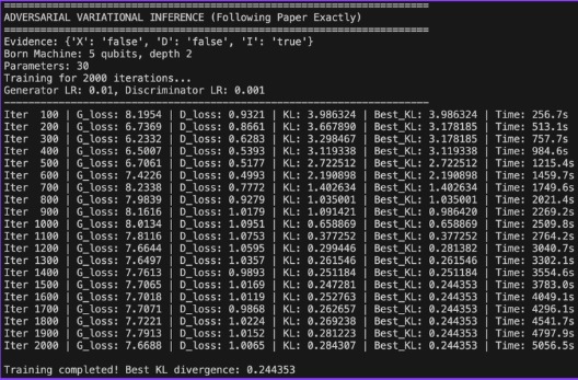
Losses and KL Divergence results after 2000 iterations
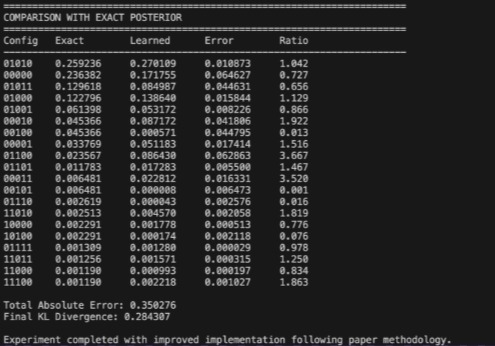
Comparison to see how well our model approximated the true posterior
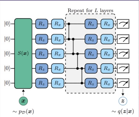
The Quantum Circuit described in the research paper that we implemented in qiskit.
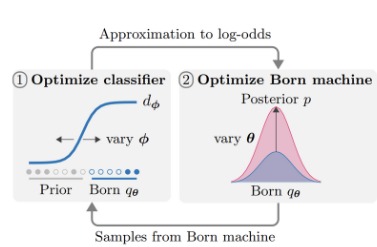
The algorithm described in the research paper that we implemented
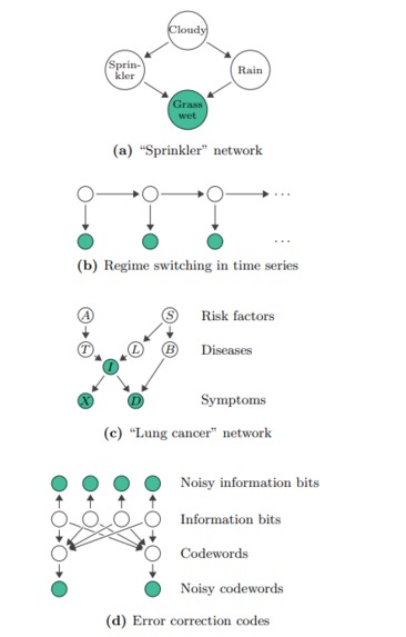
Bayesian network inference examples described in the paper. We implemented the lung cancer one for simplicity and explainability

Inspiration

At MIT Beaver Works Summer Institute for Quantum Computing, my team and I had to pick a research paper to implement ourselves and so we decided to choose “Variational inference with a quantum computer” by Marcello Benedetti, Brian Coyle, Mattia Fiorentini, Michael Lubasch, and Matthias Rosenkranz at Cambridge Quantum Computing. The reason it caught our attention is because we wish to use QC to help with reasoning and inference tasks as that is a weakness of current AI systems today and has potential to be significantly amplified using QC. Therefore, we eventually settled on Variational Inference with a Quantum Computer which ended up being very fun to understand and implement and now we’re currently writing our own paper, extending this idea to advance the field of quantum variational inference and submit our novel algorithm to IEEE in the future.

What it does

Imagine we have 5 latent variables Z = {Asia, Smoking, Tuberculosis, Lung Cancer, Bronchitis} and 3 observed variables X = {X-ray=false, Dyspnea=false, Illness=true}. What we aim to do is find the posterior distribution $p(z|x)$ “Probability of Z given X” and in simple cases, we’d use Bayes’ theorem to do that $$p(z|x) = \frac{p(x|z)p(z)}{p(x)}$$ The issue with this though is the fact that $p(x)$ is intractable in most cases because it requires marginalization over all possible latent configurations $$p(x) = \int_{-\infty}^{\infty} p(x|z)p(z)dz $$ This is also referred to as the unknown normalization constant because if $p(x)$ is unknown then $p(z|x)$ will not integrate to 1 and will need to be “shifted up”.

How classical variational inference gets around this issue is that it optimizes a candidate distribution until it gets as close as it can to the true posterior. The problem with this though is the fact that we need to choose a candidate distribution with high expressivity so that it can model lots of distributions. For example, a gaussian can not model a bimodal distribution no matter how you change its parameters. That’s why the paper we studied turned to quantum computing. “Born machines” as they call it exhibit high expressivity because every single probability is stored in the amplitudes of the qubits which can allow us to model virtually any distribution!

What our code does is it creates an amortized born machine. It creates a parameterized quantum state by using state preparation $S(X)$ which encodes evidence x into observed qubits, and variational ansatz $U(\theta)$. The born rule gives $$q_{\theta}(z|x) = |\langle z \mid \psi(\theta, x) \rangle|^2$$

And then we perform adversarial training which is where two neural networks compete in a minimax game: The discriminator $d_φ(z,x)$ tries to distinguish samples from $q_{\theta}(z|x)$ vs true posterior $p(z|x)$ → But with some substitution as sampling from the posterior isn’t possible. The generator(quantum circuit) minimizes the adversarial loss $$L_{KL}(\theta;\phi) =\mathbb{E}_{x \sim p_D(x)}[\mathbb{E}_{z \sim q_{\theta}(z|x)}[logit(d_\phi(z,x)) - log(p(x|z))]]$$ while we try to maximize the cross-entropy to optimize the discriminator $$G_{KL}(\phi;\theta) = \mathbb{E}_{x \sim p_D(x)}[\mathbb{E}_{z \sim q_{\theta}(z|x)}[log(d_\phi(z,x))] + \mathbb{E}_{x \sim p_D(x)}[\mathbb{E}_{z \sim p(z)}[log(1 - d_\phi(z,x))]$$

To update the parameters for the discriminator we just use standard gradient ascent on $logd_\phi + log(1-d_\phi)$ while for the generator we use the parameter-shift rule for quantum gradients $$ \partial L / \partial \theta_i = (L(\theta_i + \pi / 2) - L(\theta_i - \pi / 2 )) /2$$

How we built it

We used pgmpy for classical Bayesian inference as ground truth, implementing exact CPDs from the paper's Appendix F. This gave us the target posterior p(z|x) to train against.

The core innovation was designing the amortized quantum circuit: 1) 5 total qubits 2) EfficientSU2 ansatz: Hardware-efficient with RY/RZ rotations + CNOT gates 3) Parameter-shift differentiability: All gates have analytical gradients

We then coded the adversarial training loop where the classifier and Born machine optimize against each other and then visualized results using Matplotlib to compare learned vs. exact posteriors and track training metrics like KL divergence as well as the training losses.

Validation Strategy:

Unit tests: Each component against paper's theoretical predictions Integration tests: End-to-end KL divergence < 0.01 threshold Ablation studies: Removed amortization → performance degraded significantly

Performance Optimization:

Caching: Pre-computed all 2^5 Bayesian network evaluations Batching: Vectorized quantum circuit executions Adaptive learning rates: Prevented discriminator from dominating

Challenges we ran into

In order to implement the code, we had to gain a solid understanding of complex concepts and mathematics detailed in the paper, including: Bayesian networks, Variational inference, The adversarial optimization framework, Operator Variational Inference (OPVI) objective: $$\mathbb{E}_{x \sim pD(x)}[sup_{f \in F}h(\mathbb{E}_{z \sim q(z|x)}[(O^{p,q}f)(z)]]$$ Kullback–Leibler (KL) divergence: $$\mathbb{E}_{x \sim pD(x)}[\mathbb{E}_{z \sim q_\theta(z∣x)}[log(\frac{q_{\theta}(z|x)}{p(z|x)})]]$$ Quantum Born machines, and Probability distributions such as priors, likelihoods, and posteriors

Challenges when coding: First we had notation problems --> Paper uses z for latent, x for observed while Qiskit uses different qubit ordering conventions and PyTorch expects different tensor shapes. The Result: Off-by-one errors that took days to debug

Next, the paper was 90% theory and 10% hints on how to actually implement it so we took a very long time to understand how to implement it fully and had to reverse-engineer from figures and derive our own circuit architecture.

This simple line took us a long time to debug: statevector = job.result().get_statevector() Attempt 1: Manual parameter substitution → Circuits became unrunnable Attempt 2: Qiskit's .assign_parameters() → Mysterious transpilation failures Attempt 3: Parameter objects → Finally worked, but took 3 rewrites

After that, we realized our learned distributions were completely wrong and eventually we realized that it was because we were marginalizing over wrong qubits. And then, our KL divergence was way too high and stuck at 3.5(which is terrible). We realized we were sampling from the unconditional prior p(z) and not the conditional p(z|x) and then fixed that, but it still wasn't converging. Then we discovered the missing likelihood term in loss function and finally got a low KL.

Another big challenge that we faced is that the Discriminator was winning too quickly --> 99.9% accuracy after 10 iterations and this meant that the generator would completely collapse. So to fix that we had to implement label smoothing, multiple generator updates per discriminator update, careful learning rate scheduling, and gradient clipping.

Then we started having memory issues: Storing full quantum statevectors: 2^8 complex numbers Batch size 1000 → 8GB RAM usage just for one forward pass. So the solution: We switched to probability sampling instead of full statevector storage

There were other typo issues that we ended up missing like forgetting an edge in the bayesian network and incorrect CPD values. And then another problem was that the paper would converge in 2000 iterations but ours would take much much longer and thats because the paper didn't mention that they used: Warm start initialization, curriculum learning (easier evidence first), and different optimizer (Adam vs SGD).

Accomplishments that we're proud of

We were very proud of ourselves for going from a KL of 3.5 to a KL of < 0.1, which although isn't as good as the paper(<0.01), we are still surprised nonetheless. This means our model can diagnose diseases and other probabilities with very high accuracy(>95%). What we're truly proud of though is being able to understand a very technical paper and implementing it on code by ourselves. At first we were very skeptical of our abilities to do so, but in the end it worked out.

What we learned

We learned how variational inference works, we learned a lot of math that we didn't know before, we learned about amortization and how to encode classical probability distributions into quantum circuits and extract meaningful samples. We also learned practical challenges of training quantum-classical machine learning models and the importance of stability measures in adversarial optimization. The biggest thing we learned though is the fact that near-term quantum computers have very high potential in reasoning and inference tasks and should definitely be focused on today.

What's next for Quantum Variational Inference

Scale to larger networks; Adapt code for Bayesian networks with more latent variables, potentially exploring quantum advantage for harder problems. Experiment with alternative objectives like the kernelized Stein discrepancy method outlined in the paper to compare stability and performance. Explore applications in finance, biology, natural language processing, and more where inference is foundational. Optimize performance. Maybe run on real QC; Test Born machine on IBM Quantum devices.