ISRO recently released the full archive of medium and low-resolution Earth Observation dataset to the public. This includes the imagery from LISS-IV camera aboard ResourceSat-2 and ResourceSat-2A satellites. This is currently the highest spatial resolution imagery available in the public domain for India. In this post, I want to cover the steps required to download the imagery and apply the pre-processing steps required to make this data ready for analysis – specifically how to programmatically convert the DN values to TOA Reflectance. We will use modern Python libraries such as XArray, rioxarray, and dask – which allow use to seamlessly work with large datasets and use all the available compute power on your machine.

Downloading Data

The LISS4 imagery archive is accessible via ISRO’s EO Data Hub – Bhoonidhi. Users must create a free account and login to download the scenes. The image below shows the steps required to search the open data around your chosen location, preview the results and download the scenes.

The scenes come as a zip file containing GeoTIFF files for each spectral band. Here is some key information about the imagery.

• Number of Bands: 3 (Green, Red, and NIR)
• Spatial Resolution: 5.8m
• Radiometric Resolution: 10-bits
• Swath: 70km
• Temporal Resolution: 24 days (While the camera system is capable of 5-day revisit time over targeted areas – the systematic combined acquisition with ResourceSat2 and 2A in multispectral mode is 24-days)
• Coverage: India (Scenes outside India are available by order, not as a direct download)
• Archive: 2011-current

Processing the Data

We will use Python to process the downloaded scene into a stacked 3-band Cloud-Optimized GeoTIFF files with TOA Reflectance. The source data is quite large and traditional computing methods are not efficient is processing it effectively. Libraries like rasterio will read the entire image into RAM and you are likely to run out of memory when processing the entire scene. You are also limited to using a single CPU and cannot use multiprocessing to distribute the work to multiple cores or machines.

A modern approach to working with large rasters is to use XArray. XArray is designed to work with dimensional raster datasets and natively supports parallel-computing with Dask. With minimal configuration, you can leverage all the cores on your machine for parallel computing. The rioxarray extension makes it possible to work with geospatial rasters using XArray. In this example, we will build a workflow to process the raw LISS4 scene into an analysis-ready stacked GeoTIFF.

Installation and Configuration

My preferred method of installing and managing Python packages is using conda. We create a new environment and install the required packages. We are also using the PyEphem package to obtain the Earth-Sun distance that can be installed using pip.

conda create --name liss4
conda activate liss4
conda install -c conda-forge rioxarray dask jupyterlab -y
pip install ephem

Once installed, start a new Jupyter Notebook and import the required packages.

import datetime
import ephem
import math
import os
import rioxarray as rxr
import xarray as xr
import zipfile

Next we initiate a local dask cluster. This uses all the available cores on your machine in parallel. You will see a link to the Dask Dashboard. We will use this dashboard later in this tutorial.

from dask.distributed import Client, progress
client = Client()  # set up local cluster on the machine
client

We are now ready to start the data processing.

Extract and Read Metadata

We first unzip the scene zip file to a folder.

with zipfile.ZipFile(liss4_zip) as zf:
  # The LISS4 zip files contain a folder with all the data
  # Get the folder name
  foldername = [
      info.filename for info in zf.infolist()
      if info.is_dir()][0]
  # Extract all the data
  zf.extractall()

print(f'Extracted the files to {foldername}.')

Each scene contains a file named BAND_META.txt containing the scene metadata. We parse the file and extract the data as a Python dictionary.

metadata_filename = 'BAND_META.txt'
metadata_filepath = os.path.join(foldername, metadata_filename)

metadata = {}
with open(metadata_filepath) as f:
  for line in f:
    key, value = line.split('=')
    metadata[key.strip()] = value.strip()

scene_id = metadata['OTSProductID']
print(f'Metadata extracted successfully for scene: {scene_id}')

Read and Stack Bands

LISS4 images come as 3 individual GeoTIFF rasters for each band. The image files are named BAND2.tif, BAND3.tif and BAND4.tif . We read them using rioxarray. Here we set chunks=True indicating that we want to use Dask and split the dataset into smaller chunks that can be processed in parallel.

b2_path = os.path.join(foldername, 'BAND2.tif')
b3_path = os.path.join(foldername, 'BAND3.tif')
b4_path = os.path.join(foldername, 'BAND4.tif')

b2_ds = rxr.open_rasterio(b2_path, chunks=True)
b3_ds = rxr.open_rasterio(b3_path, chunks=True)
b4_ds = rxr.open_rasterio(b4_path, chunks=True)

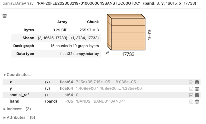
Create a XArray Dataset by stacking individual band images. The scene has a NoData value of 0. So we set the correct NoData value before further processing.

scene = xr.concat(
    [b2_ds, b3_ds, b4_ds], dim='band').assign_coords(
    band=['BAND2', 'BAND3', 'BAND4']
)

scene = scene.where(scene != 0)
scene.name = scene_id
scene

Converting DN to Reflectances

The pixel values of the source images are DN values that need to be converted to reflectances before they can be used for analysis.

The correction formulae and sensor parameters are published in the following paper

Sharma, Anu & Badarinath, K. & Roy, Parth. (2008). Corrections for atmospheric and adjacency effects on high resolution sensor data a case study using IRS-P6 LISS-IV data. https://www.isprs.org/proceedings/xxxvii/congress/8_pdf/3_wg-viii-3/05.pdf

acq_date_str = metadata['DateOfPass']
# Date is in the format 04-MAR-2023
acq_date = datetime.datetime.strptime(
    acq_date_str, '%d-%b-%Y')

sun_elevation_angle = metadata['SunElevationAtCenter']
sun_zenith_angle = 90 - float(sun_elevation_angle)

We need to compute the Earth-Sun distance at the date of acquisition. We use the pyephm library to obtain this.

observer = ephem.Observer()
observer.date = acq_date
sun = ephem.Sun()
sun.compute(observer)
d = sun.earth_distance

Define the Saturation Radiance for each band. These come from the RESOURCESAT-2 Data Users’ Handbook and are available in metadata as well.

b2_sr = 53.0
b3_sr = 47.0
b4_sr = 31.5

Define ex-atmospheric solar irradiance values for each band ESUN for each band as published in At-sensor Solar Exo-atmospheric Irradiance, Rayleigh Optical Thickness and Spectral parameters of RS-2 Sensors.

b2_esun = 181.89
b3_esun = 156.96
b4_esun = 110.48

Define other contants needed for computation.

pi = math.pi
sun_zenith_angle_rad = math.radians(sun_zenith_angle)

Convert DN to Radiance

b2_dn = scene.sel(band='BAND2')
b3_dn = scene.sel(band='BAND3')
b4_dn = scene.sel(band='BAND4')

b2_rad = b2_dn*b2_sr/1024
b3_rad = b3_dn*b3_sr/1024
b4_rad = b4_dn*b4_sr/1024

Convert Radiance to TOA Reflectance

b2_ref = (pi*b2_rad*d*d)/(b2_esun*math.cos(sun_zenith_angle_rad))
b3_ref = (pi*b3_rad*d*d)/(b3_esun*math.cos(sun_zenith_angle_rad))
b4_ref = (pi*b4_rad*d*d)/(b4_esun*math.cos(sun_zenith_angle_rad))

Stack the bands into a single XArray Dataset.

reflectance_bands = [b2_ref, b3_ref, b4_ref]
scene_ref = xr.concat(
    reflectance_bands, dim='band').assign_coords(
    band=['BAND2', 'BAND3', 'BAND4']
).chunk('auto')
scene_ref.name = scene_id
scene_ref

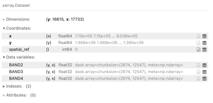
Write Results to Disk

Our DataArray is structured to have ‘band’ as a dimension which makes it easy for data manipulation and processing. But for use in standard GIS software – it is better to create an XArray Dataset with each band as a variable.

output_ds = scene_ref.to_dataset('band')
output_ds

Define the options for the output file. We use the COG driver to create a Cloud-Optimized GeoTIFF file.

output_file = f'{scene_id}.tif'

output_options = {
    'driver': 'COG',
    'compress': 'deflate',
    'num_threads': 'all_cpus',
    'windowed': False # set True if you run out of RAM
}

Write the raster.

output_ds[['BAND2', 'BAND3', 'BAND4']].rio.to_raster(
    output_file, **output_options)
print(f'Output file created {output_file}')

Dask will now run the processing graph on the local cluster. So far, no computation has happened. We defined the processing steps which created a task graph that will be used to perform a series of tasks to compute the final result. Each step can be computed in parallel by distributing the ‘chunk’ of data to different workers. In our case, they will be distributed to different CPU cores. Once you run the cell to create the output raster, visit the Dask Dashboard on your machine (Typically at http://127.0.0.1:8787/status ) to see the computation being carried out.

View the Result

The final stacked image with TOA reflectance will be written to the disk once the processing is finished. Here’s what the resulting image looks like in QGIS.

We can change the band combination to create a False Color Composite. Here we are displaying the BAND4, BAND3 and BAND2 in Red, Green and Blue channels to create NRG composite.

Here’s a zoomed-in view of the image.

Below is a comparison of LISS4 data vs. Sentinel-2 images of the same region. You can see the fine-scale details due to the 5.8m spatial resolution of LISS4 vs. 10m spatial resolution of Sentinel-2.

Summary

The goal of this post was to document a Python workflow for pre-processing LISS4 imagery along with demonstrating the use of state-of-the-art open-source computing techniques. You can check out the Full Notebook on GitHub or Run the Notebook on Colab with a demo dataset.

If you have feedback or corrections – please leave a comment below.