Binomial Distribution in NumPy
Last Updated :
05 Dec, 2025
The Binomial Distribution models the number of successes in a fixed number of independent trials where each trial has only two outcomes: success or failure. In NumPy, we use the numpy.random.binomial() method to generate values that follow this distribution. It is commonly used in coin flips, defect detection, surveys, and probability experiments.
Example: Here, we generate one binomial random value using 10 trials and a 0.5 probability of success.
Python
import numpy as np
x = np.random.binomial(n=10, p=0.5)
print(x)
Explanation: np.random.binomial(n=10, p=0.5) simulates 10 yes/no events and returns how many times success occurred.
Syntax
numpy.random.binomial(n, p, size=None)
Parameters:
- n: Number of trials
- p: Probability of success in each trial
- size: Shape of output array
Examples
Example 1: In this example, we generate 5 binomial random numbers using 10 trials and 0.5 probability.
Python
import numpy as np
arr = np.random.binomial(n=10, p=0.5, size=5)
print(arr)
Explanation: np.random.binomial(..., size=5) returns an array of 5 simulated outcomes.
Example 2: Here, we simulate 8 trials with different success probability (p = 0.3).
Python
import numpy as np
x = np.random.binomial(8, 0.3, size=4)
print(x)
Explanation: np.random.binomial(8, 0.3) generates values where success occurs with 30% probability.
Example 3: In this example, we generate a 2×3 matrix of binomial outcomes.
Python
import numpy as np
m = np.random.binomial(12, 0.6, size=(2, 3))
print(m)
Explanation: size=(2,3) creates a 2D array where each entry is a binomial random value.
Visualizing the Binomial Distribution
Visualizing the generated numbers helps in understanding their behavior. Below is an example of plotting a histogram of random numbers generated using numpy.random.binomial.
Python
import numpy as np
import matplotlib.pyplot as plt
from scipy.stats import binom

n = 10
p = 0.5
size = 1000

data = np.random.binomial(n, p, size)

plt.hist(data, bins=np.arange(-0.5, n+1.5, 1), density=True, edgecolor='black', alpha=0.7, label='Histogram')

x = np.arange(0, n+1)
pmf = binom.pmf(x, n, p)

plt.scatter(x, pmf, color='red', label='Theoretical PMF')
plt.vlines(x, 0, pmf, colors='red', linestyles='dashed')

plt.title("Binomial Distribution (n=10, p=0.5)")
plt.xlabel("Number of Successes")
plt.ylabel("Probability")
plt.legend()
plt.grid(True)
plt.show()
Output
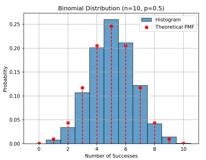 Binomial Distribution Plot
Explanation:
- np.random.binomial(n, p, size) generates 1000 simulated outcomes.
- plt.hist(..., density=True) shows the frequency distribution of these values.
- binom.pmf(x, n, p) computes the theoretical probability for each possible success count.
- Red dots and dashed lines show the true Binomial PMF for comparison.
Explore
Introduction
Creating NumPy Array
NumPy Array Manipulation