This post is a record of my struggles learning the Lean 4 Proof Assistant, which I’m doing by the inefficient and misleading strategy of interpreting it whenever I can as a souped-up version of Haskell.
Curry–Howard in propositional logic
The formula

is the generic instance of the second axiom scheme in Lukasiewicz’s formulation of propositional logic. As such, it is a tautology, true under any assignment of true and false to the propositional letters. An elegant proof of this is by the Curry–Howard correspondence for propositional logic: a proposition is a tautology if and only if, interpreting the propositional letters as type variables, there is a function of the corresponding type. Thus the fact that the Haskell compiler accepts
lukasiewicz2 :: (p -> (q -> r))

    -> ((p -> q) -> (p -> r))

lukasiewicz2 h_ptoqr h_pq h_p = (h_ptoqr h_p) (h_pq h_p)

-- h_ptoqr h_p :: q -> r evaluated at h_pq h_p :: q ...

-- has type r
or that the Lean compiler accepts
lemma lukasiewicz2 {p q r : Prop} : (p → (q → r))

    → ((p → q) → (p → r))

  := fun h_ptoqr h_pq h_p => (h_ptoqr h_p) (h_pq h_p)
is a proof that the Lukasiewicz formula is a tautology. Here h_pq can be read as ‘the hypothesis that 
lemma lukasiewicz2' {p q r : Prop}

    (h_ptoqr : p → (q → r)) (h_pq : p → q) : p → r

  := fun h_p => (h_ptoqr h_p) (h_pq h_p)
This proof can be rewritten in tactic style using the intro tactic to introduce the hypothesis h_p of type p, and then the exact tactic to finish:
lemma lukasiewicz2'' {p q r : Prop}

    (h_ptoqr : p → (q → r)) (h_pq : p → q) : p → r

  := by intro h_p; exact (h_ptoqr h_p) (h_pq h_p)
One thing I am struggling with in Lean is to get used to tactics, so examples like this where the macro-rewriting black box can easily be understood are particularly welcome. I hope the not so-subtle neurolinguistic programming of typing fun every so often will keep me motivated.
Some more tautologies
In a similar spirit, the Curry–Howard proofs that p → p and p → (q → p) are tautologies have one word solutions: id (valid in Haskell and Lean), and const (valid in Haskell). Here p → (q → p) is the generic instance of the first Lukasiewicz axiom scheme.
Negation
In Lean, negation is definitionally the same as ‘implies false’. That is 
data False, to introduce a new type False which deliberately does not have any constructors. We then define negation by the type synonym type Not p = p -> False. (As a visual aid, -> is the Haskell arrow; this is allowed by Lean, but Lean also supports → which I’ve used for all Lean code.) For example, the proposition 
impossible :: (p, Not p) -> False

impossible (h_p, h_notp) = h_notp h_p
given by evaluating the function h_notp :: p → False at h_p :: p. One could curry this definition to get the equivalent tautology 
impossible' h_p h_notp = h_notp h_p. The analogous Lean code for the curried form is
lemma impossible {p : Prop} : p → ¬p → False

  := fun h_p => fun h_np => h_np h_p
which, very similarly to before, can be rewritten as
lemma impossible' {p : Prop} (h_p : p) (h_np : ¬p)

  : False := h_np h_p
Observe that since a proposition cannot be both true and false, it is impossible, without using the special Haskell value undefined, or its Lean colleague sorry, to construct two valid inputs to impossible. (Or for another proof of this, note that a successful evaluation of impossible gives a value of the void type False.) But still, the fact that impossible type checks confirms that it is a tautology.
For a simpler instance, observe that id :: False → False type checks and so 


p is itself a void type, in which case we have 
id is the unique function of type False → False.
The contrapositive and vector space duality
Continuing in this mathematical theme, the contrapositive, formulated so that it introduces rather than removes a negation, is 
contrapositive :: (p -> q) -> (Not q -> Not p)

contrapositive h_pq h_nq h_p = h_nq (h_pq h_p)
is a valid Haskell program, that takes h_pq : p -> q and the proof that p is false, as expressed by a value of type h_nq : q -> False, to produce a new value, namely the composition h_nq . h_pq of type p -> False, which is then evaluated at h_p : p, the argument of the output Not p. Here it may be helpful to note that the final parentheses are redundant: the type could also be written as (p -> q) -> (q -> False) -> (p -> False). Again the Lean code is almost identical:
lemma contrapositive {p q : Prop} : (p → q) → (¬q → ¬p)

  := fun h_pq h_nq h_p => h_nq (h_pq h_p)

  -- fun h_pq => (fun h_nq => (fun h_p =>

  --       h_nq (h_pq h_p)))
where the commented out lines are the less idiomatic form; like any civilised being, Lean curries by default.
The flip in the direction of implication corresponds to vector space duality: if we read False as 


double_negation_intro :: p -> Not (Not p)

  -- equivalently p -> (p -> False) -> False

double_negation_intro h_p h_np = h_np h_p
or in Lean
lemma double_negation_intro {p : Prop} : p → ¬¬p

  := fun h_p => (fun h_notp => h_notp h_p)
which works because ¬¬p is (p → False) → False so we can take the given value of type p and evaluate it at the argument of type p → False. As an antidote to the false argument that the number of negations cannot go down, I find it helpful to consider
lemma triple_negation_elimination {p : Prop} : ¬¬¬p → ¬p

  := fun h_nnnp =>

    (fun h_p => h_nnnp (double_negation_intro h_p))
which corresponds to the canonical map 


As a big hint for the question at the following section, can you define a map 

Double negation elimination
The Lukasiewicz system needs a third axiom scheme to become complete, in the sense that all tautologies are provable from the axioms by repeated applications of modus ponens. This third axiom scheme has as its generic instance the contrapositive, this time removing negation:

Does this have a Curry–Howard proof in Haskell? Does it have a Curry–Howard proof in Lean? Using the version of the contrapositive already proved, we can certainly prove 


The Curry–Howard proof of this in Haskell is, using our existing functions,
lukasiewicz3_nearly :: (Not p -> Not q)

  -> q -> Not (Not p)

lukasiewicz3_nearly h_npnq h_q =

  contrapositive h_npnq (double_negation_intro h_q)
which can be ‘desugared’ in careful steps to
lukasiewicz3_nearly1 h_npnq h_q = \h_nq ->

  contrapositive h_npnq (double_negation_intro h_q) h_nq

lukasiewicz3_nearly2 h_npnq h_q = \h_nq ->

  (double_negation_intro h_q) (h_npnq h_nq)

lukasiewicz3_nearly3 h_npnq h_q = \h_nq ->

  (\h_nq' -> h_nq' h_q) (h_npnq h_nq)

lukasiewicz3_nearly4 h_npnq h_q = \h_nq

  -> (h_npnq h_nq) h_q

lukasiewicz3_nearly5 h_npnq h_q h_nq = h_npnq h_nq h_q
I find it quite remarkable that, without a type signature, the inferred type for the final version is (a -> b -> c) -> b -> a -> c, which by parametric polymorphism and the theorems for free mantra, has unique value
lukasiewicz3_nearly6 g x y = g y x
I have no intuition for why this apparently complicated tautology involving both negation and double negation should be such a simple combinator.
It is now clear that the third Lukasiewicz axiom scheme is equivalent in logical power to double negation elimination. But, finally reaching one punchline, the Haskell type Not (Not p) -> p, and its syntactic equivalent ((p -> False) -> False) -> p are uninhabited. Thus there is no way to complete
double_negation_elimination :: Not (Not p) -> p

double_negation_elimination h_nnp = ...
without using undefined. Thus Haskell exhibits the Curry–Howard logic for intuitionistic, rather than classical, logic.
The foundations of Lean are in homotopy type theory, which is also intuitionistic. But Lean supports classical logic, and if I understand right, this is automatically enabled by importing Mathlib. Remembering that proof by contradiction is ‘the falsity of 

lemma double_negation_elimination {p : Prop} :

  ¬¬p → p := by_contra

  -- by_contra has type (¬?m.1 → False) → ?m.1
If you are playing along and find this gives an error, please add import Mathlib.Tactic.ByContra at the top of your file. Or add import Mathlib, and go away and make some tea. I used a full import of Mathlib for the examples of dependent types involving natural numbers below. Using this we can prove the instance of the third Lukasiewicz scheme:
lemma contrapositive_eliminating_negation {p q : Prop}

  : (¬p → ¬q) → q → p :=

  fun h_npnq h_q => by by_contra h_np;

  -- we have h_npnq : ¬p → ¬q, h_q : q and now h_np : ¬p

  -- so all set up for

  exact h_npnq h_np h_q
where the definition in the body could be rewritten as intro h_npnq h_q; by_contra h_np; exact h_npnq h_np h_q
Peirce’s Law
For a similar example, Peirce’s Law, that 
call-with-current-continuation. This type is void in Haskell: instead the nearest approximation is callCC
class Monad m => MonadCont m where

  callCC :: ((a -> m b) -> m a) -> m a
where, omitting type constructors, and choosing a fixed return type r, one suitable type for a monad in the class MonadCont is m p = (p -> r) -> r. This might suggest taking r to be False but then m a is Not (Not a), so we stay in the doubly negated world. I found it an instructive exercise to deduce double negation elimination from Peirce’s Law, by using Peirce with 


sorry in the sublemma h_aux : ¬¬p → (¬p → p) below as an exercise. As a hint, one solution begins with intro h_nn h_n to get hold of values of the input types ¬¬p and \neg p; now compare the earlier proof by contradiction.
lemma peirce_implies_double_negation_elimination

  : (∀ r q : Prop, ((r → q) → r) → r)

          → (∀ p : Prop, ¬¬p → p) := by

  intro peirce p

  specialize peirce p False

  -- current state is p : Prop, peirce :

    ((p → False) → p) → p, goal ¬¬p → p

  have h_aux : ¬¬p → (¬p → p) := by sorry

  exact fun h_nnp => peirce (h_aux h_nnp)
This proof is probably comically long-winded to experts but no matter. At least I now have a better appreciation for why the first year undergraduates doing my introduction to pure maths course used to write proofs that began with a confident ‘suppose for a contradiction’, continued with a contrapositive, flirted perhaps with induction, and so on and so on, until eventually one reached the meat of the proof, which was usually a one line direct proof of the required proposition.
Types of types
Whereas in Haskell there are values, types and kinds (but without extensions the only kind that matters is 
[1,2,3] or the string literal "hello". As in Haskell, these values have various types, for instance Nat for 3, ℝ for 1.234, List Nat for [1,2,3] and String for "hello". (Unlike Haskell, strings are not definitionally the same as lists of characters, so String is more like Haskell’s efficient Text data type.) Thus 3 : Nat, 1.234 : ℝ, [1,2,3] : List Nat and "hello" : String. Each of Nat, ℝ, List Nat, String is a type. The common type of all these types is Type, which can also be notated Type 0. The hierarchy then proceeds: the type of Type is Type 1, the type of Type 1 is Type 2, and so on. Off to one side, but at the lowest level of all, are values of a further type: Prop. This is the only type we have used so far. The type of Prop is Type. Thus
         10 : Nat   : Type : Type 1 : Type 2

h_p : p → p : Prop : Type : Type 1 : Type 2
are chains of valid type signatures (supposing that h_p and p are in scope) and
variable (p q : Prop)

#check p → (q → p)

#check p → q

#check p → p
prints out p → (q → p) : Prop, p → q : Prop, and p → p : Prop, as expected. (Note the second is not an inhabited type.) To avoid having to inspect the interactive output, one can include the expected output at the end, using an extra pair of parentheses. Thus
#check (p → (q → p) : Prop)
is a suitable replacement for the first check; any mismatch gets highlighted in VSCode with the usual red cross. Some of the claims above on types of types can be confirmed using
#check (3 : Nat)

#check (Nat : Type)

#check (Prop : Type)

#check (Type : Type 1)
Impredicativity of the proposition type
One subtle point is that normally the type of a function α → β where α : Type i, β : Type j is Type k where k is the maximum of i and j. But if β : Prop then no matter how high α is in the hierarchy, the resulting type is Prop. Thus the types of the entity following := in the three examples below are respectively Type 2, Prop and Prop
example {α : Type 1} {β : Type 2} : Type 2 := α → β

example : Prop := (n : Nat) → 0 + n = n

example {p : Prop} : Prop := (α : Type 4) → p
This property ‘impredicativity of Prop‘ is needed below so that our functions of dependent type are propositions, and so compound proofs do not quickly leave the world of propositions.
Proof irrelevance
I have the strong feeling that there can be essentially different proofs of the same proposition. For example, the Fundamental Theorem of Algebra can be proved by induction on the 2-power dividing the degree of the polynomial, using only the intermediate value theorem from basic calculus, or instead as a corollary of Liouville’s theorem from complex analysis that a bounded entire function is constant. Lean 4 would disagree:
theorem proof_irrelevance {p : Prop} (h_p h'_p : p)

  : h_p = h'_p := by rfl
Here rfl can, I think, be read as ‘are reflexively equal’. The analogue in Haskell would be a data type P that is made an instance of Eq by instance Eq P where _ == _ = True.
Aside on curly braces in types
The block {p q r : Prop} in the first example lukasiewicz2 declares that p, q, r are implicitly of type Prop; this block can be omitted, if one first declares variable (p q r : Prop) at the top of the file, as in the check example above. This is a bit like declaring p, q, r to be global types, each themselves of type Prop; compare a global declaration const int x = 3 of global values in a traditional imperative language such as C. Lean also has an analogue of Haskell’s type classes, for which square brackets are used. For instance [Ring R] means that the compiler should know (probably from some other file) that R has the structure of a ring. We won’t need type classes at all below.
Function types and forall
So far we have stayed in the world of propositional logic (which unlike predicate logic does not have quantification), and correspondingly, except for double-negation elimination, everything we have done in Lean can also be done in Haskell. Function types, or 

∀ (r : Prop), r → r : Prop for both the #check queries below.
#check (r : Prop) → r → r

#check ∀ r : Prop, r → r
This is not the same as the output p → p : Prop of #check p → p, which is only valid thanks to the variable declaration variable (p q : Prop) above. Thus ∀ r : Prop, r → r is the type of functions whose
- first argument is a proposition, called
r(say) - return value has type the proposition
r → r
Or equivalently, ∀ r : Prop, r → r is the type of functions whose
- first argument is a proposition, called
r(as it happens) - second argument is a value of type
r(let’s call ith_r) - returning a value of type
r(it must beh_r).
As confirmation here are Lean proofs of the axiom 
lemma self_implication {p : Prop} : p → p := id

lemma self_implication' : (∀ r : Prop, r → r) :=

  by intro r; exact id

lemma self_implication'' : (r : Prop) → r → r :=

  fun r h_r => h_r
Both primed forms have identical type signatures (when read by the compiler) and the values defined, i.e. the identity functions r → r for each r : Prop are definitionally equivalent. The compiler, at least with my default settings, will object that the argument p in the final function form is unused; it is a nice touch that the output is still more cluttered by the instruction set_option linter.unusedVariables false on how to declutter it. But fair enough: it would be more idiomatic to write
lemma self_implication''' : (r : Prop) → r → r :=

  fun _ h_r => h_r
using the same underscore notation as Haskell for the ‘function hole’. Yet further definitions (i.e. the part following :=) are possible, for instance,
lemma self_implication'''' : (r : Prop) → r → r :=

  by simp

lemma self_implication''''' : (r : Prop) → r → r :=

  by simp?
both succeed, and the latter even tells us how it did it:
Try this: [apply] simp only [imp_self, implies_true]
Well, if you really must. I think I prefer the identity function.
Dependent types
Observe that the type of the output of self_implication'' depends explicitly on the first argument: in the first slot p, of type Prop, is the proposition to be shown to imply itself, whereas in the second and third slots, p is the type. The nearest we can get to the type signature in Haskell, supposing a type Prop is defined, is
self_implication_Haskell :: Prop → p → p -- what's p?
except this entirely fails to capture that p is not just a proposition, but in fact the first argument of the function. Instead the type signature above specifies a function taking an arbitrary proposition to a fully polymorphic function p → p, with no connection between the type variable p and the proposition. (To underline this point, equivalent Haskell type signatures in which p appears within the scope of a universal quantifier are :: Prop -> forall p. p -> p and forall p. Prop -> p -> p; you might need to enable the language extension ExplicitForAll for this to be accepted, but it seems that it is on by default in ghci-9.6.7.) Of course since we can give a Curry–Howard proof of self-implication in Haskell, there is an acceptable definition of self_implication_Haskell, namely \lambda _ h_p = h_p, but from our new dependent-type perspective, this is just a potentially confusing stroke of good luck.
Propositions indexed by natural numbers as a dependent type
For an example where it is not just the type signature but the whole function that cannot be realised in Haskell (at least without special tricks, see the final section below), we consider propositions parametrised by natural numbers. The following are equivalent declarations of a function that takes as input a natural number n, of type Nat, and returns a value of type 0 + n = n, i.e. a proof that adding zero to n gives n.
lemma zero_add_nat : ∀ n : Nat, 0 + n = n := by sorry

lemma zero_add_nat' : (n : Nat) → (0 + n = n) :=

  by sorry
In both cases one suitable replacement for sorry is intro n; ring_nf; after introducing n, the target is 0 + n = n, which falls to the ring normal form tactic. Showing a better appreciation of MathLib, we could also use intro n; exact zero_add n, or, showing a better appreciation of Peano arithmetic, we could use
lemma zero_add_nat'' : (n : Nat) → 0 + n = n := by

  intro n; cases n

  -- zero case 0 + 0 = 0

  exact (add_zero 0)

  -- succ case: ⊢ 0 + (n' + 1) = n' + 1

  rename_i n

  -- Nat.add_assoc (n m k : ℕ) : n+m+k = n+(m+k)

  rewrite [← Nat.add_assoc]

  -- goal is now 0 + n + 1 = n + 1

  -- which is implicitly (0 + n) + 1 = n + 1

  rewrite [zero_add_nat'' n]

  rfl
Above I edited the Lean output to use n' rather than the dagger from Lean, which did not come through well on WordPress. It would be more idiomatic to replace cases n with induction n hn, where hn is bound to the inductive hypothesis. Also it is standard to use rw rather than rewrite, combining multiple rewrites in one line. Since rw includes a weak form of rfl, the final line is then redundant. With these changes we get something you might recognise from the Lean Number Game.
lemma zero_add_nat''' : (n : Nat) → 0 + n = n := by

  intro n; induction n with

  | zero => exact (add_zero 0)

  | succ n hn => rw [← Nat.add_assoc, hn]
This is also a good example of the impredicativity of Prop mentioned in the section above on the type hierarchy, where we saw that example : Prop := (n : Nat) → 0 + n = n type checks. Correspondingly, the type of the function type zero_add_nat is Prop. This can be verified, taking great care not to confuse types on the left of := with types (as values) on the right, by
def type_of_zero_add_nat := ∀ n : Nat, 0 + n = n

#check (type_of_zero_add_nat : Prop)
Pi-types
Returning to the type signatures, notice that both zero_add_nat : (n : Nat) -> 0 + n = n and
lemma self_implication''' : (p : Prop) → p → p

  := fun _ h_p => h_p
taken verbatim from above are of the general form
lemma piTest {N : Type} {f : N → Prop} : (n : N) → f n

  := by sorry
which does indeed type check. (The triangle warning is from the use of sorry, which is of course the only way to complete the definition.) For more on the 

This is the end of the Lean part of this post, and probably a very good place to stop reading. Thank you for getting this far!
Playing the natural number game in Haskell with singletons
There is a website out there with about 25 ‘design patterns’, all of which as far as I can tell are ingenious ways to work around the limitations of the type systems in more traditional languages, of which the prime miscreant seems to be Java. So it is with some dismay that I learned from the wonderful Haskell Unfolder podcast that the singleton design pattern is a good way to bring some of the expressiveness of dependent types to Haskell.
We define Peano naturals as a data type
data Nat = Zero | Succ Nat deriving (Eq, Show)
If like me, you often mistype a constructor when you mean a type, as in makeZero :: Zero as opposed to the correct makeZero :: Nat (with definition makeZero = Zero) then you will have got rather used to seeing variations on the theme of ‘Not in scope: type constructor or class ‘Zero’. A data constructor of that name is in scope; did you mean DataKinds?’ Well the great moment has finally arrived, when we do, in fact, mean DataKinds! (Seriously though, this is a nice example of why shipping without a million extensions enabled is the right choice for producing understandable error messages.) Using this extension, we get access to type level naturals, written as 'Zero,
type One = 'Succ 'Zero
and so on. Confusingly the quotes can be omitted, because (unlike this poor human) the compiler always knows what is at the value level and what is at the type level. Here I am including the quotes every time they are appropriate. The three further extensions required appear as comments in the next code block.
To encode the proposition 


data Add :: Nat -> Nat -> Nat -> Type where

  -- Uses GADTs and KindSignatures

  AddZero :: Add m 'Zero m

  AddSucc :: Add m n p -> Add m ('Succ n) ('Succ p)


deriving instance Show (Add m n p)

deriving instance Eq (Add m n p)

-- Uses StandaloneDeriving
We now use the Haskell compiler to prove that 

zeroAdd :: (n : Nat) -> Add Zero n n such that zeroAdd n has type Add Zero n n. But note that in zeroAdd n, n is a value, whereas in Add Zero n n it is a type. Thus the type of the output depends on a value in the input, exactly as expected for a dependent type. And this is not possible in Haskell, no matter how many extensions one turns on.
What we need is a bridge from values to types. For instance, we need a value of type SomeNewDataType One such that, when we pattern match on it, we know that the type parameter is One (and not ‘Zero, or ‘Succ ‘Succ ‘Zero, or …). This is what singletons do for us.
data TypeValueDict (n :: Nat) where

  TVZero :: TypeValueDict 'Zero

  TVSucc :: TypeValueDict n -> TypeValueDict ('Succ n)
As an illustration of the bridge, I offer
showTypeFromDict :: TypeValueDict nType

  -> String

showTypeFromDict TVZero = "'Zero"

showTypeFromDict (TVSucc nValue) =

  "'Succ " ++ showTypeFromDict nValue


tvOneTypeString = showTypeFromDict

  (TVSucc TVZero :: TypeValueDict One)

  -- no quote for One, it is a type (well really a Nat)
where the output is the string "'Succ 'Zero'"; earlier we declared One as a type synonym for 'Succ 'Zero; it has type Nat
The proof that zeroAdd :: (n : Nat) -> Add Zero n n is made legitimate using the dictionary.
zeroAdd :: TypeValueDict n -> Add Zero n n

zeroAdd TVZero     = AddZero

zeroAdd (TVSucc r) = AddSucc (zeroAdd r)


zeroAddOne = zeroAdd (TVSucc TVZero) ::  Add Zero One One
The fact that this compiles is a proof, at the type level, that


 Posted by mwildon
 for `aesthetic merit’. You can read Gemini’s solution verbatim in the evaluation report linked above.
  to be the number of
  -dimensional subspaces of
  . If
. If  or
or  then, by definition, the
  for a varying
  -dimensional subspace that is counted in part of the proof; if the subspace is instead fixed, often as part of the hypotheses, we use
  .
. be a given
  . The number of
  .
. be the canonical basis of
 . There are
  choices for each of
  and so
 followed by a basis for
  we obtain a matrix
 correspond to distinct subspaces
  is
is  .
. is an
is an  -dimensional subspace of
  containing
  . Hence there are
  -choices for a subspace
  in which
  -dimensional subspace
  .
. be given
  -dimensional subspace of
  . The number of
  is
is  .
. , there are
  complementary subspaces
  to
to  . Now again use that subspaces of the quotient space
  are in bijection with subspaces of
 -dimensional subspace
  of
of  having intersection of dimension
  with
with  and
and  , there are
  such subspaces. Summing over
  gives the result.
  , else
 and
and  in the original version, cancel in a few places, swap the order of the binomial coefficients in each product, and then erase the primes.
  induced by applying the unit on
  to get a canonical inclusion
  .
. defined by
  maps to ‘evaluate at
 ![v \stackrel{\eta_V}{\longmapsto} [\theta \mapsto \theta(v)]\qquad(\star)](https://s0.wp.com/latex.php?latex=v+%5Cstackrel%7B%5Ceta_V%7D%7B%5Clongmapsto%7D+%5B%5Ctheta+%5Cmapsto+%5Ctheta%28v%29%5D%5Cqquad%28%5Cstar%29&bg=ffffff&fg=333333&s=0&c=20201002)
 and
and  . Thus
  defines a natural transformation
  from the identity functor on Vect to the double dual functor
  . This will turn out out to to be the unit in the double dual monad.
 is a vastly bigger vector space than
  is the vector space of all
  . Moreover
  . (Even the existence of bases for
  it is implied by the Boolean Prime Ideal Theorem, a weak form of the Axiom of Choice.) For this reason we have to reason formally, mainly by manipulating symbols, rather than use matrices or bases. But this is a good thing: for instance it means our formulae for the monad unit and monad multiplication translates entirely routinely to define the continuation monad in the category Hask.
 . Thus for each vector space
  . As already said, we obtain this as the dual map to
  . That is
 is the linear map
 ![\theta \stackrel{\eta_{V^\star}}{\longmapsto} [\phi \mapsto \phi(\theta)]](https://s0.wp.com/latex.php?latex=%5Ctheta+%5Cstackrel%7B%5Ceta_%7BV%5E%5Cstar%7D%7D%7B%5Clongmapsto%7D+%5B%5Cphi+%5Cmapsto+%5Cphi%28%5Ctheta%29%5D&bg=ffffff&fg=333333&s=0&c=20201002)
 and
and  . Generally, given a linear map
  , the dual map is given by `restriction along
  ‘: that is, we regard a dual vector
  as an element of
  by mapping
  into
into  by
by  ; in symbols
  . Therefore the dual map to
  , is
, is![w \stackrel{\mu_V}{\longmapsto} [\theta \mapsto w(\eta_{V^\star}(\theta))] = [\theta \mapsto w([\phi \mapsto \phi(\theta)])] \quad (\dagger)](https://s0.wp.com/latex.php?latex=w+%5Cstackrel%7B%5Cmu_V%7D%7B%5Clongmapsto%7D+%5B%5Ctheta+%5Cmapsto+w%28%5Ceta_%7BV%5E%5Cstar%7D%28%5Ctheta%29%29%5D+%3D+%5B%5Ctheta+%5Cmapsto+w%28%5B%5Cphi+%5Cmapsto+%5Cphi%28%5Ctheta%29%5D%29%5D++%5Cquad+%28%5Cdagger%29&bg=ffffff&fg=333333&s=0&c=20201002)

 ; multiplication then becomes the observation that interpreting variables in a boolean formula as yet further boolean formulae does not leave the space of boolean formulae. Here I will note that the definition of
  in
in  does at least typecheck:
  is an element of
  and therefore in the domain of
  . Naturality of
 defines a monad. For this we need to check the monad laws shown in the commutative diagrams below.
 . This has a short proof, which, as expected from the remark about formalism above, come down to juggling the order of symbols until everything works out. Recall that
  is the canonical embedding of
  . Thus if we take
  is the element of
  defined by
 . This map sends
 ![[\phi \mapsto \phi(\theta)]](https://s0.wp.com/latex.php?latex=%5B%5Cphi+%5Cmapsto+%5Cphi%28%5Ctheta%29%5D&bg=ffffff&fg=333333&s=0&c=20201002) in
in ![\begin{aligned} (\mu_V \circ \eta_{V^{\star\star}})(\phi) &= \mu_V([\Psi \mapsto \Psi(\phi)]) \\&= [\theta \mapsto (\eta_{V^\star}(\theta))(\phi)] \\ &= [\theta \mapsto \phi(\theta)] \\&= \phi \end{aligned}](https://s0.wp.com/latex.php?latex=%5Cbegin%7Baligned%7D+%28%5Cmu_V+%5Ccirc+%5Ceta_%7BV%5E%7B%5Cstar%5Cstar%7D%7D%29%28%5Cphi%29+%26%3D+%5Cmu_V%28%5B%5CPsi+%5Cmapsto+%5CPsi%28%5Cphi%29%5D%29+%5C%5C%26%3D+%5B%5Ctheta+%5Cmapsto+%28%5Ceta_%7BV%5E%5Cstar%7D%28%5Ctheta%29%29%28%5Cphi%29%5D+%5C%5C+%26%3D+%5B%5Ctheta+%5Cmapsto+%5Cphi%28%5Ctheta%29%5D+%5C%5C%26%3D+%5Cphi+%5Cend%7Baligned%7D&bg=ffffff&fg=333333&s=0&c=20201002)
 is indeed the identity of
  , I will omit it. I plan in a sequel to this post to show that
  is the monad induced by the adjunction betweeen the contravariant dual and itself; the identity monad law then becomes the
  for the right-hand functor
  in the adjunction, and the associativity law becomes an immediate application of the
  is some kind of linear map
  , and since all we have to hand is
  itself? It would be intriguing if this could be made into a rigorous argument either working in Vect or directly in Hask, perhaps using ideas from Wadler’s paper
  , as defined in
  to
to![\mu_V(w) = [\theta \mapsto w(\eta_{V^\star}(\theta))]](https://s0.wp.com/latex.php?latex=%5Cmu_V%28w%29+%3D+%5B%5Ctheta+%5Cmapsto+w%28%5Ceta_%7BV%5E%5Cstar%7D%28%5Ctheta%29%29%5D&bg=ffffff&fg=333333&s=0&c=20201002) to
to  or unpacked fully,
 ![f^{\star\star}\phi = [\theta \mapsto \phi(f^\star (\theta))] = \theta \mapsto \phi(\theta \circ f)](https://s0.wp.com/latex.php?latex=f%5E%7B%5Cstar%5Cstar%7D%5Cphi+%3D+%5B%5Ctheta+%5Cmapsto+%5Cphi%28f%5E%5Cstar+%28%5Ctheta%29%29%5D+%3D+%5Ctheta+%5Cmapsto+%5Cphi%28%5Ctheta+%5Ccirc+f%29&bg=ffffff&fg=333333&s=0&c=20201002)
 .
. , but surely the input won’t be, but the true reason is to make a distinction between the types
  and then
  is evaluated, and so on. (This can be checked using the linked Haskell code, which puts a trace on plus.) Still bad, but more easily fixed, is the left-associative fold
  , and then
  is evaluated, and so on. The correct way to write it uses a strict left-fold, available as
  , and otherwise we modify the continuation so that it first adds
  . Note that although this might look like a left-associative fold, it does the same computation as the right-associative fold.
  by sampling from
  . From my mental picture of the bell curve, I think it is intuitive that the mean of the resulting sample will be not much more than
 . More precisely, it is
 of the standard normal distribution.
  , we have
 should be well approximated by an exponential distribution with parameter
  , and, correspondingly, as is
  . Thus this approximation suggests that the mean of the tail distribution should be
  and its variance
  or more standard deviations from the mean, in a sample conditioned to be at least
  outliers
 and you have 50 colleagues, then since only 2.3% of the conditioned sample are outliers, lying in the
  tail, there is a good chance that none of your colleagues is more than 1 standard deviation ahead of you in ability.
 we sample from
  (lucky people). Suppose that
  is small, say
  , so the effect of luck is relatively modest, boosting one’s performance by just
  a standard deviation. As before, we then reject all samples below the threshold
  of being lucky. The final column is the ratio of lucky to average people.
 tail of the distribution (with, as just explained, a boost of 0.5 for lucky people), lucky people predominate. The effect is that the University of Erewhon fails in its goal of recruiting people three standard deviations above the mean: instead of the 2230 successful candidate, 1176 are people who are merely about 2.5 standard deviations above the mean, but happened to get lucky.
 random variable, so the standard deviation is
  distribution, the effect is to increase the variance, while leaving the mean unchanged. The graphs below show the probability density function for the original
  tail, for
  .
. 

 (the blue curve) only 10.09% of the conditional probability density function is in the negative half. Almost everyone recruited gets lucky, most by at least one standard deviation from the mean and many by two or more standard deviations from the mean. The moral is again clear: unless you believe (as is sometimes
 is the number of
  to a long exact sequence of polynomial representations of
  , working over an arbitrary field
  . We then descend to get quick proofs of generalizations of the symmetric function identity
 and the corresponding
  , namely
![\sum_{r=0}^n (-1)^r q^{r(r-1)2} \genfrac{[}{]}{0pt}{}{n-r+D-1}{n-r}_q \genfrac{[}{]}{0pt}{}{D}{r}_q = 0.](https://s0.wp.com/latex.php?latex=%5Csum_%7Br%3D0%7D%5En+%28-1%29%5Er+q%5E%7Br%28r-1%292%7D+%5Cgenfrac%7B%5B%7D%7B%5D%7D%7B0pt%7D%7B%7D%7Bn-r%2BD-1%7D%7Bn-r%7D_q++%5Cgenfrac%7B%5B%7D%7B%5D%7D%7B0pt%7D%7B%7D%7BD%7D%7Br%7D_q+%3D+0.&bg=ffffff&fg=333333&s=0&c=20201002)
 denote the number of
 . I finish by explaining how my
  over an arbitrary field
  , we define its weight, denoted
  , to be its sum of entries. We shall adopt a slightly unconventional approach and define the
 ![\genfrac{[}{]}{0pt}{}{n}{k}_q \in \mathbb{C}[q]](https://s0.wp.com/latex.php?latex=%5Cgenfrac%7B%5B%7D%7B%5D%7D%7B0pt%7D%7B%7D%7Bn%7D%7Bk%7D_q+%5Cin+%5Cmathbb%7BC%7D%5Bq%5D&bg=ffffff&fg=333333&s=0&c=20201002) to be the enumerator by weight of the
to be the enumerator by weight of the  , normalized to have constant term
  . That is,
![\genfrac{[}{]}{0pt}{}{n}{k}_q = q^{-k(k-1)/2} \sum_{X \subseteq \{0,1,\ldots, n-1\}} q^{\mathrm{wt}(X)}.](https://s0.wp.com/latex.php?latex=%5Cgenfrac%7B%5B%7D%7B%5D%7D%7B0pt%7D%7B%7D%7Bn%7D%7Bk%7D_q+%3D+q%5E%7B-k%28k-1%29%2F2%7D+%5Csum_%7BX+%5Csubseteq+%5C%7B0%2C1%2C%5Cldots%2C+n-1%5C%7D%7D+q%5E%7B%5Cmathrm%7Bwt%7D%28X%29%7D.&bg=ffffff&fg=333333&s=0&c=20201002)
![\genfrac{[}{]}{0pt}{}{n}{k}_q = 0](https://s0.wp.com/latex.php?latex=%5Cgenfrac%7B%5B%7D%7B%5D%7D%7B0pt%7D%7B%7D%7Bn%7D%7Bk%7D_q+%3D+0&bg=ffffff&fg=333333&s=0&c=20201002) if
if ![\genfrac{[}{]}{0pt}{}{n}{k}_q](https://s0.wp.com/latex.php?latex=%5Cgenfrac%7B%5B%7D%7B%5D%7D%7B0pt%7D%7B%7D%7Bn%7D%7Bk%7D_q&bg=ffffff&fg=333333&s=0&c=20201002) is a polynomial in
is a polynomial in ![\begin{aligned} \genfrac{[}{]}{0pt}{}{4}{2}_q&= q^{-1}(q^{0+1} + q^{0+2} + q^{0+3} + q^{1+2} + q^{1+3} + q^{2+3}) \\ &= 1 + q + 2q^2 + q^3 + q^4, \end{aligned}](https://s0.wp.com/latex.php?latex=%5Cbegin%7Baligned%7D+%5Cgenfrac%7B%5B%7D%7B%5D%7D%7B0pt%7D%7B%7D%7B4%7D%7B2%7D_q%26%3D+q%5E%7B-1%7D%28q%5E%7B0%2B1%7D+%2B+q%5E%7B0%2B2%7D+%2B+q%5E%7B0%2B3%7D+%2B+q%5E%7B1%2B2%7D+%2B+q%5E%7B1%2B3%7D+%2B+q%5E%7B2%2B3%7D%29+%5C%5C+%26%3D+1+%2B+q+%2B+2q%5E2+%2B+q%5E3+%2B+q%5E4%2C+%5Cend%7Baligned%7D&bg=ffffff&fg=333333&s=0&c=20201002)
![\genfrac{[}{]}{0pt}{}{n}{0}_q = \genfrac{[}{]}{0pt}{}{n}{n}_q = 1](https://s0.wp.com/latex.php?latex=%5Cgenfrac%7B%5B%7D%7B%5D%7D%7B0pt%7D%7B%7D%7Bn%7D%7B0%7D_q+%3D+%5Cgenfrac%7B%5B%7D%7B%5D%7D%7B0pt%7D%7B%7D%7Bn%7D%7Bn%7D_q+%3D+1&bg=ffffff&fg=333333&s=0&c=20201002) and
and ![\genfrac{[}{]}{0pt}{}{n}{1}_q = 1 + q + \cdots + q^{n-1}](https://s0.wp.com/latex.php?latex=%5Cgenfrac%7B%5B%7D%7B%5D%7D%7B0pt%7D%7B%7D%7Bn%7D%7B1%7D_q++%3D+1+%2B+q+%2B+%5Ccdots+%2B+q%5E%7Bn-1%7D&bg=ffffff&fg=333333&s=0&c=20201002) for all
for all  . We now recover the usual definition of
  , which we prove by adapting the standard bijective proof.
 then
then![\genfrac{[}{]}{0pt}{}{n}{k}_q = q^{n-k} \genfrac{[}{]}{0pt}{}{n-1}{k-1}_q + \genfrac{[}{]}{0pt}{}{n-1}{k}_q.](https://s0.wp.com/latex.php?latex=%5Cgenfrac%7B%5B%7D%7B%5D%7D%7B0pt%7D%7B%7D%7Bn%7D%7Bk%7D_q+%3D+q%5E%7Bn-k%7D+%5Cgenfrac%7B%5B%7D%7B%5D%7D%7B0pt%7D%7B%7D%7Bn-1%7D%7Bk-1%7D_q++%2B+%5Cgenfrac%7B%5B%7D%7B%5D%7D%7B0pt%7D%7B%7D%7Bn-1%7D%7Bk%7D_q.&bg=ffffff&fg=333333&s=0&c=20201002)
 then the result holds by our convention that
 ![\genfrac{[}{]}{0pt}{}{n-1}{-1}_q = 0](https://s0.wp.com/latex.php?latex=%5Cgenfrac%7B%5B%7D%7B%5D%7D%7B0pt%7D%7B%7D%7Bn-1%7D%7B-1%7D_q+%3D+0&bg=ffffff&fg=333333&s=0&c=20201002) so we may suppose that
so we may suppose that  . Removing
  from a
  containing
  subsets of
  , enumerated by
 ![\genfrac{[}{]}{0pt}{}{n-1}{k-1}_q](https://s0.wp.com/latex.php?latex=%5Cgenfrac%7B%5B%7D%7B%5D%7D%7B0pt%7D%7B%7D%7Bn-1%7D%7Bk-1%7D_q&bg=ffffff&fg=333333&s=0&c=20201002) . This map decreases the weight by
. This map decreases the weight by ![\genfrac{[}{]}{0pt}{}{n-1}{k}_q](https://s0.wp.com/latex.php?latex=%5Cgenfrac%7B%5B%7D%7B%5D%7D%7B0pt%7D%7B%7D%7Bn-1%7D%7Bk%7D_q&bg=ffffff&fg=333333&s=0&c=20201002) . Therefore,
. Therefore, ![q^{k(k-1)/2} \genfrac{[}{]}{0pt}{}{n}{k}_q = q^{n-1} q^{(k-1)(k-2)/2} \genfrac{[}{]}{0pt}{}{n-1}{k-1}_q + q^{k(k-1)/2} \genfrac{[}{]}{0pt}{}{n-1}{k}_q.](https://s0.wp.com/latex.php?latex=q%5E%7Bk%28k-1%29%2F2%7D+%5Cgenfrac%7B%5B%7D%7B%5D%7D%7B0pt%7D%7B%7D%7Bn%7D%7Bk%7D_q+%3D+q%5E%7Bn-1%7D+q%5E%7B%28k-1%29%28k-2%29%2F2%7D+%5Cgenfrac%7B%5B%7D%7B%5D%7D%7B0pt%7D%7B%7D%7Bn-1%7D%7Bk-1%7D_q+%2B+q%5E%7Bk%28k-1%29%2F2%7D+%5Cgenfrac%7B%5B%7D%7B%5D%7D%7B0pt%7D%7B%7D%7Bn-1%7D%7Bk%7D_q.&bg=ffffff&fg=333333&s=0&c=20201002)
 , using that
![[n]_q](https://s0.wp.com/latex.php?latex=%5Bn%5D_q&bg=ffffff&fg=333333&s=0&c=20201002) by
by ![[n]_q = 1 + q + \cdots + q^{n-1}](https://s0.wp.com/latex.php?latex=%5Bn%5D_q+%3D+1+%2B+q+%2B+%5Ccdots+%2B+q%5E%7Bn-1%7D&bg=ffffff&fg=333333&s=0&c=20201002) and the quantum factorial
and the quantum factorial ![[n]_q!](https://s0.wp.com/latex.php?latex=%5Bn%5D_q%21&bg=ffffff&fg=333333&s=0&c=20201002) by
by ![[n]_q! = [n]_q[n-1]_q \ldots [1]_q](https://s0.wp.com/latex.php?latex=%5Bn%5D_q%21+%3D+%5Bn%5D_q%5Bn-1%5D_q+%5Cldots+%5B1%5D_q&bg=ffffff&fg=333333&s=0&c=20201002) . Observe that specializing
. Observe that specializing  , respectively. (See the section on characters below for the connection with the alternative convention in which quantum numbers are Laurent polynomials.) Note that in the following proposition, if
 ![\genfrac{[}{]}{0pt}{}{n}{0}_q = 1](https://s0.wp.com/latex.php?latex=%5Cgenfrac%7B%5B%7D%7B%5D%7D%7B0pt%7D%7B%7D%7Bn%7D%7B0%7D_q+%3D+1&bg=ffffff&fg=333333&s=0&c=20201002) for all
for all ![\displaystyle\genfrac{[}{]}{0pt}{}{n}{k}_ q = \frac{[n]_q[n-1]_q \ldots [n-k+1]_q}{[k]_q!}.](https://s0.wp.com/latex.php?latex=%5Cdisplaystyle%5Cgenfrac%7B%5B%7D%7B%5D%7D%7B0pt%7D%7B%7D%7Bn%7D%7Bk%7D_+q+%3D+%5Cfrac%7B%5Bn%5D_q%5Bn-1%5D_q+%5Cldots+%5Bn-k%2B1%5D_q%7D%7B%5Bk%5D_q%21%7D.&bg=ffffff&fg=333333&s=0&c=20201002)
 using the previous lemma we have
![\begin{aligned} \genfrac{[}{]}{0pt}{}{n}{k}_q &= q^{n-k}\genfrac{[}{]}{0pt}{}{n-1}{k-1}_q + \genfrac{[}{]}{0pt}{}{n-1}{k}_q \\ &= q^{n-k} \frac{[n-1]_q\ldots [n-k+1]_q[n-k]_q}{[k-1]_q!} \\ &\qquad \qquad \qquad + \frac{[n-1]_q\ldots [n-k+1]_q[n-k]_q}{[k]_q!} \\&= \frac{[n-1]_q\ldots [n-k+1]_q}{[k]_q!} \bigl( q^{n-k}[k]_q + [n-k]_q \bigr) \\ &= \frac{[n-1]_q \ldots [n-k+1]_q}{[k]_q!} [n]_q \\ \end{aligned}](https://s0.wp.com/latex.php?latex=%5Cbegin%7Baligned%7D+%5Cgenfrac%7B%5B%7D%7B%5D%7D%7B0pt%7D%7B%7D%7Bn%7D%7Bk%7D_q+%26%3D++q%5E%7Bn-k%7D%5Cgenfrac%7B%5B%7D%7B%5D%7D%7B0pt%7D%7B%7D%7Bn-1%7D%7Bk-1%7D_q+%2B+%5Cgenfrac%7B%5B%7D%7B%5D%7D%7B0pt%7D%7B%7D%7Bn-1%7D%7Bk%7D_q+%5C%5C+%26%3D+q%5E%7Bn-k%7D+%5Cfrac%7B%5Bn-1%5D_q%5Cldots+%5Bn-k%2B1%5D_q%5Bn-k%5D_q%7D%7B%5Bk-1%5D_q%21%7D+%5C%5C+%26%5Cqquad+%5Cqquad+%5Cqquad+%2B+%5Cfrac%7B%5Bn-1%5D_q%5Cldots+%5Bn-k%2B1%5D_q%5Bn-k%5D_q%7D%7B%5Bk%5D_q%21%7D+%5C%5C%26%3D+%5Cfrac%7B%5Bn-1%5D_q%5Cldots+%5Bn-k%2B1%5D_q%7D%7B%5Bk%5D_q%21%7D+%5Cbigl%28++q%5E%7Bn-k%7D%5Bk%5D_q+%2B+%5Bn-k%5D_q++%5Cbigr%29+%5C%5C+%26%3D+%5Cfrac%7B%5Bn-1%5D_q+%5Cldots+%5Bn-k%2B1%5D_q%7D%7B%5Bk%5D_q%21%7D+%5Bn%5D_q+%5C%5C+%5Cend%7Baligned%7D&bg=ffffff&fg=333333&s=0&c=20201002)
![\begin{aligned} q^{n-k}[k]_q + [n-k]_q &= q^{n-k}(1+q + \cdots + q^{k-1}) \\ & \qquad\qquad + 1 + q + \cdots + q^{n-k-1} \\ &= 1 + q + \cdots + q^{n-1} \\&= [n]_q \end{aligned}](https://s0.wp.com/latex.php?latex=%5Cbegin%7Baligned%7D+q%5E%7Bn-k%7D%5Bk%5D_q+%2B+%5Bn-k%5D_q+%26%3D+q%5E%7Bn-k%7D%281%2Bq+%2B+%5Ccdots+%2B+q%5E%7Bk-1%7D%29++%5C%5C+%26+%5Cqquad%5Cqquad+%2B+1+%2B+q+%2B+%5Ccdots+%2B+q%5E%7Bn-k-1%7D+%5C%5C+%26%3D+1+%2B+q+%2B+%5Ccdots+%2B+q%5E%7Bn-1%7D+%5C%5C%26%3D+%5Bn%5D_q+%5Cend%7Baligned%7D&bg=ffffff&fg=333333&s=0&c=20201002)
![\left[\!\genfrac{[}{]}{0pt}{}{n}{k}\!\right]_q = \sum_M q^{\mathrm{wt}(M)}](https://s0.wp.com/latex.php?latex=%5Cleft%5B%5C%21%5Cgenfrac%7B%5B%7D%7B%5D%7D%7B0pt%7D%7B%7D%7Bn%7D%7Bk%7D%5C%21%5Cright%5D_q+%3D+%5Csum_M+q%5E%7B%5Cmathrm%7Bwt%7D%28M%29%7D&bg=ffffff&fg=333333&s=0&c=20201002)
![\begin{aligned} \left[\!\genfrac{[}{]}{0pt}{}{3}{2}\!\right]_q &= q^{0+0} + q^{0+1} + q^{0+2} + q^{1+1} + q^{1+2} + q^{2+2} \\ &= 1 + q + 2q^2 + q^3 + q^4 \\ &= \genfrac{[}{]}{0pt}{}{4}{2}_q\end{aligned}](https://s0.wp.com/latex.php?latex=%5Cbegin%7Baligned%7D+%5Cleft%5B%5C%21%5Cgenfrac%7B%5B%7D%7B%5D%7D%7B0pt%7D%7B%7D%7B3%7D%7B2%7D%5C%21%5Cright%5D_q++%26%3D+q%5E%7B0%2B0%7D+%2B+q%5E%7B0%2B1%7D+%2B+q%5E%7B0%2B2%7D+%2B+q%5E%7B1%2B1%7D+%2B+q%5E%7B1%2B2%7D+%2B+q%5E%7B2%2B2%7D+%5C%5C+%26%3D+1+%2B+q+%2B+2q%5E2+%2B+q%5E3+%2B+q%5E4++%5C%5C+%26%3D+%5Cgenfrac%7B%5B%7D%7B%5D%7D%7B0pt%7D%7B%7D%7B4%7D%7B2%7D_q%5Cend%7Baligned%7D+&bg=ffffff&fg=333333&s=0&c=20201002)
![\left[\!\genfrac{[}{]}{0pt}{}{n}{0}\!\right]_q = 1](https://s0.wp.com/latex.php?latex=%5Cleft%5B%5C%21%5Cgenfrac%7B%5B%7D%7B%5D%7D%7B0pt%7D%7B%7D%7Bn%7D%7B0%7D%5C%21%5Cright%5D_q+%3D+1&bg=ffffff&fg=333333&s=0&c=20201002) and
and![\left[\!\genfrac{[}{]}{0pt}{}{n}{1}\!\right]_q = q^0 + q^1 + \cdots + q^{n-1} = [n]_q = \genfrac{[}{]}{0pt}{}{n}{1}_q](https://s0.wp.com/latex.php?latex=%5Cleft%5B%5C%21%5Cgenfrac%7B%5B%7D%7B%5D%7D%7B0pt%7D%7B%7D%7Bn%7D%7B1%7D%5C%21%5Cright%5D_q+%3D+q%5E0+%2B+q%5E1+%2B+%5Ccdots+%2B+q%5E%7Bn-1%7D+%3D+%5Bn%5D_q+%3D+%5Cgenfrac%7B%5B%7D%7B%5D%7D%7B0pt%7D%7B%7D%7Bn%7D%7B1%7D_q&bg=ffffff&fg=333333&s=0&c=20201002)
![\left[\!\genfrac{[}{]}{0pt}{}{3}{2}\!\right]_q = \genfrac{[}{]}{0pt}{}{4}{2}_q](https://s0.wp.com/latex.php?latex=%5Cleft%5B%5C%21%5Cgenfrac%7B%5B%7D%7B%5D%7D%7B0pt%7D%7B%7D%7B3%7D%7B2%7D%5C%21%5Cright%5D_q+%3D+%5Cgenfrac%7B%5B%7D%7B%5D%7D%7B0pt%7D%7B%7D%7B4%7D%7B2%7D_q&bg=ffffff&fg=333333&s=0&c=20201002) is not a coincidence.
is not a coincidence. where
where  . In turn, such sequences are in bijection with
  by the map
 to a subset of weight
  . By the first section,
 ![q^{k(k-1)/2}\genfrac{[}{]}{0pt}{}{n+k-1}{k}_q](https://s0.wp.com/latex.php?latex=q%5E%7Bk%28k-1%29%2F2%7D%5Cgenfrac%7B%5B%7D%7B%5D%7D%7B0pt%7D%7B%7D%7Bn%2Bk-1%7D%7Bk%7D_q&bg=ffffff&fg=333333&s=0&c=20201002) enumerates
enumerates ![\left[\!\genfrac{[}{]}{0pt}{}{n}{k}\!\right]_q = \genfrac{[}{]}{0pt}{}{n+k-1}{k}_q .\qquad(2)](https://s0.wp.com/latex.php?latex=%5Cleft%5B%5C%21%5Cgenfrac%7B%5B%7D%7B%5D%7D%7B0pt%7D%7B%7D%7Bn%7D%7Bk%7D%5C%21%5Cright%5D_q+%3D+%5Cgenfrac%7B%5B%7D%7B%5D%7D%7B0pt%7D%7B%7D%7Bn%2Bk-1%7D%7Bk%7D_q+.%5Cqquad%282%29+&bg=ffffff&fg=333333&s=0&c=20201002)
![\left[\!\genfrac{[}{]}{0pt}{}{n}{k}\!\right]_q](https://s0.wp.com/latex.php?latex=%5Cleft%5B%5C%21%5Cgenfrac%7B%5B%7D%7B%5D%7D%7B0pt%7D%7B%7D%7Bn%7D%7Bk%7D%5C%21%5Cright%5D_q&bg=ffffff&fg=333333&s=0&c=20201002) . Observe that a partition whose Young diagram is contained in the
. Observe that a partition whose Young diagram is contained in the  box is uniquely specified by the sequence
  of
of  adds
adds  . Therefore
 corresponds to recording a partition not by the
  and
and  of the partitions
  and
and  are shown in the diagram below with step numbers in bold.
![\genfrac{[}{]}{0pt}{}{n}{k}_q = q^{n-k} \genfrac{[}{]}{0pt}{}{n-1}{k-1}_q + \genfrac{[}{]}{0pt}{}{n-1}{k}_q.](https://s0.wp.com/latex.php?latex=%5Cgenfrac%7B%5B%7D%7B%5D%7D%7B0pt%7D%7B%7D%7Bn%7D%7Bk%7D_q+%3D++q%5E%7Bn-k%7D+%5Cgenfrac%7B%5B%7D%7B%5D%7D%7B0pt%7D%7B%7D%7Bn-1%7D%7Bk-1%7D_q+%2B+%5Cgenfrac%7B%5B%7D%7B%5D%7D%7B0pt%7D%7B%7D%7Bn-1%7D%7Bk%7D_q.&bg=ffffff&fg=333333&s=0&c=20201002)
![\genfrac{[}{]}{0pt}{}{n}{k}_q = \genfrac{[}{]}{0pt}{}{n-1}{k-1}_q + q^k \genfrac{[}{]}{0pt}{}{n-1}{k}_q.](https://s0.wp.com/latex.php?latex=%5Cgenfrac%7B%5B%7D%7B%5D%7D%7B0pt%7D%7B%7D%7Bn%7D%7Bk%7D_q+%3D+%5Cgenfrac%7B%5B%7D%7B%5D%7D%7B0pt%7D%7B%7D%7Bn-1%7D%7Bk-1%7D_q+%2B+q%5Ek+%5Cgenfrac%7B%5B%7D%7B%5D%7D%7B0pt%7D%7B%7D%7Bn-1%7D%7Bk%7D_q.&bg=ffffff&fg=333333&s=0&c=20201002)
![(1 + qz)(1+q^2 z) \ldots (1+q^{n-1}z) = \sum_{k=0}^n q^{k(k-1)/2} \genfrac{[}{]}{0pt}{}{n}{k}_q z^k](https://s0.wp.com/latex.php?latex=%281+%2B+qz%29%281%2Bq%5E2+z%29+%5Cldots+%281%2Bq%5E%7Bn-1%7Dz%29+%3D+%5Csum_%7Bk%3D0%7D%5En+q%5E%7Bk%28k-1%29%2F2%7D+%5Cgenfrac%7B%5B%7D%7B%5D%7D%7B0pt%7D%7B%7D%7Bn%7D%7Bk%7D_q+z%5Ek&bg=ffffff&fg=333333&s=0&c=20201002)
 and
and  be the elementary and complete symmetric functions of degree
  . Thus
  denote the Schur function labelled by the partition
  as defined combinatorially by
 entries of
  for each
  then
then  . It is a good basic exercise to show that
  and
and  . It is immediate from our definition of
 ![e_k(1,q,\ldots, q^{n-1}) = q^{k(k-1)/2} \genfrac{[}{]}{0pt}{}{n}{k}_q](https://s0.wp.com/latex.php?latex=e_k%281%2Cq%2C%5Cldots%2C+q%5E%7Bn-1%7D%29+%3D+q%5E%7Bk%28k-1%29%2F2%7D+%5Cgenfrac%7B%5B%7D%7B%5D%7D%7B0pt%7D%7B%7D%7Bn%7D%7Bk%7D_q&bg=ffffff&fg=333333&s=0&c=20201002)
![h_k(1,q,\ldots, q^{n-1}) = \left[\!\genfrac{[}{]}{0pt}{}{n}{k}\!\right] = \genfrac{[}{]}{0pt}{}{n+k-1}{k}_q](https://s0.wp.com/latex.php?latex=h_k%281%2Cq%2C%5Cldots%2C+q%5E%7Bn-1%7D%29+%3D+%5Cleft%5B%5C%21%5Cgenfrac%7B%5B%7D%7B%5D%7D%7B0pt%7D%7B%7D%7Bn%7D%7Bk%7D%5C%21%5Cright%5D+%3D+%5Cgenfrac%7B%5B%7D%7B%5D%7D%7B0pt%7D%7B%7D%7Bn%2Bk-1%7D%7Bk%7D_q&bg=ffffff&fg=333333&s=0&c=20201002)
![h_k(1,q,\ldots, q^{n-k}) = \genfrac{[}{]}{0pt}{}{n}{k}.](https://s0.wp.com/latex.php?latex=h_k%281%2Cq%2C%5Cldots%2C+q%5E%7Bn-k%7D%29+%3D+%5Cgenfrac%7B%5B%7D%7B%5D%7D%7B0pt%7D%7B%7D%7Bn%7D%7Bk%7D.&bg=ffffff&fg=333333&s=0&c=20201002) The
The 
 enumerates semistandard tableaux with entries from
  by their weight, i.e. their sum of entries.
 denote the Schur function labelled by the partition
  is a
is a  -dimensional vector space then the trace of the diagonal matrix with entries
  acting on
  is
is  . It is an instructive exercise to verify from this property that
  and
and  .
.  and
and  are isomorphic if and only if the specialized Schur functions
  and
and  are equal up a power of
  of
of  has character
 acting on
  ,
,  .) Restricting to
  , meaning that if
  then
then  , and so we work most naturally with Laurent polynomials in
  . (This is essential since unequal characters of
  has character

 is the plethysm product. (This is the main idea needed to prove the theorem.) One can always pass from a Laurent polynomial identity in
 ![\mathbb{C}[Q,Q^{-1}]](https://s0.wp.com/latex.php?latex=%5Cmathbb%7BC%7D%5BQ%2CQ%5E%7B-1%7D%5D&bg=ffffff&fg=333333&s=0&c=20201002) to a polynomial identity in
to a polynomial identity in ![\mathbb{C}[q]](https://s0.wp.com/latex.php?latex=%5Cmathbb%7BC%7D%5Bq%5D&bg=ffffff&fg=333333&s=0&c=20201002) polynomials by setting
polynomials by setting  and multiplying through by a suitable power of
 ![[q^a]f(z)](https://s0.wp.com/latex.php?latex=%5Bq%5Ea%5Df%28z%29&bg=ffffff&fg=333333&s=0&c=20201002) for the coefficient of
for the coefficient of  , we have
![[q^r] \genfrac{[}{]}{0pt}{}{n}{k}_q = [q^{n(n-1)/2-r}] \genfrac{[}{]}{0pt}{}{n}{k}_q](https://s0.wp.com/latex.php?latex=%5Bq%5Er%5D+%5Cgenfrac%7B%5B%7D%7B%5D%7D%7B0pt%7D%7B%7D%7Bn%7D%7Bk%7D_q+%3D+%5Bq%5E%7Bn%28n-1%29%2F2-r%7D%5D+%5Cgenfrac%7B%5B%7D%7B%5D%7D%7B0pt%7D%7B%7D%7Bn%7D%7Bk%7D_q&bg=ffffff&fg=333333&s=0&c=20201002)
 . [Hint: there is a one-line proof using
  is
is  , and that the palindromic property is preserved by multiplication and division, and then apply this to the formula in the proposition.]
 and
and  in the theorem, we obtain that the representations
  and
and  of
of ![e_k(1,q,\ldots, q^{\ell-1}) = q^{\ell(\ell-1)/2}\genfrac{[}{]}{0pt}{}{\ell}{k}_q](https://s0.wp.com/latex.php?latex=e_k%281%2Cq%2C%5Cldots%2C+q%5E%7B%5Cell-1%7D%29+%3D+q%5E%7B%5Cell%28%5Cell-1%29%2F2%7D%5Cgenfrac%7B%5B%7D%7B%5D%7D%7B0pt%7D%7B%7D%7B%5Cell%7D%7Bk%7D_q&bg=ffffff&fg=333333&s=0&c=20201002) and
and ![h_k(1,q,\ldots, q^{m-1}) = \genfrac{[}{]}{0pt}{}{m+k-1}{k}_q](https://s0.wp.com/latex.php?latex=h_k%281%2Cq%2C%5Cldots%2C+q%5E%7Bm-1%7D%29+%3D+%5Cgenfrac%7B%5B%7D%7B%5D%7D%7B0pt%7D%7B%7D%7Bm%2Bk-1%7D%7Bk%7D_q&bg=ffffff&fg=333333&s=0&c=20201002) are equal up a power of
are equal up a power of  and obtain the Wronksian isomorphism.
![\left[\!\genfrac{[}{]}{0pt}{}{n}{k}\!\right]_q = \genfrac{[}{]}{0pt}{}{n+k-1}{k}_q](https://s0.wp.com/latex.php?latex=%5Cleft%5B%5C%21%5Cgenfrac%7B%5B%7D%7B%5D%7D%7B0pt%7D%7B%7D%7Bn%7D%7Bk%7D%5C%21%5Cright%5D_q+%3D+%5Cgenfrac%7B%5B%7D%7B%5D%7D%7B0pt%7D%7B%7D%7Bn%2Bk-1%7D%7Bk%7D_q&bg=ffffff&fg=333333&s=0&c=20201002) to the level of representations. Instead going down to the level of ordinary binomial coefficients, by setting
to the level of representations. Instead going down to the level of ordinary binomial coefficients, by setting  , we obtain
 (defined as a quotient of
  is replaced with its dual
  (defined as a submodule of
  ), holds as an isomorphism of representations of
  be a
be a  -dimensional vector space over
  . Show that, regarded as a representation of
  ,
,  has
has  as an irreducible
 as a one-dimensional submodule isomorphic to the determinant representation, with quotient the irreducible
  can be thought of as the space of homogeneous polynomials of degree
  ; it is the degree
 ![\mathbb{F}[X,Y] = \bigoplus_{r \ge 0} \mathrm{Sym}^r \! E.](https://s0.wp.com/latex.php?latex=%5Cmathbb%7BF%7D%5BX%2CY%5D+%3D+%5Cbigoplus_%7Br+%5Cge+0%7D+%5Cmathrm%7BSym%7D%5Er+%5C%21+E.&bg=ffffff&fg=333333&s=0&c=20201002)
 for either side.) Thus we can identify
  with a subspace of
 ![\mathrm{Sym}_k \mathbb{F}[X,Y]](https://s0.wp.com/latex.php?latex=%5Cmathrm%7BSym%7D_k+%5Cmathbb%7BF%7D%5BX%2CY%5D&bg=ffffff&fg=333333&s=0&c=20201002) Since, given any vector space
Since, given any vector space  is the subspace of
  of symmetric tensors, we can, in turn, identify
 ![\bigl( \mathbb{F}[X,Y]\bigr)^{\otimes k}](https://s0.wp.com/latex.php?latex=%5Cbigl%28+%5Cmathbb%7BF%7D%5BX%2CY%5D%5Cbigr%29%5E%7B%5Cotimes+k%7D&bg=ffffff&fg=333333&s=0&c=20201002) spanned by the symmetrisation of all tensors
spanned by the symmetrisation of all tensors 
 . (Note that this symmetrization should be performed without introducing scalar factors, giving a basis
  ,
,  ,
,  as in the exercise above when
  and
and  .) Finally we use that this tensor product is isomorphic to
 ![\mathbb{F}[X_1,Y_1,\ldots,X_k,Y_k]](https://s0.wp.com/latex.php?latex=%5Cmathbb%7BF%7D%5BX_1%2CY_1%2C%5Cldots%2CX_k%2CY_k%5D&bg=ffffff&fg=333333&s=0&c=20201002) by the very explicit isomorphism defined on a spanning set by
by the very explicit isomorphism defined on a spanning set by .
. that are symmetric with respect to permutation of indices. It might at first seem a little strange that the non-commutative tensor product can be represented in a commutative polynomial algebra, but I think any confusion is resolved when one realises that the indices of the
 can be defined very simply by
 is all polynomials in
  with respect to each pair of variables
  denote the action of
  on the indices of a polynomial
 ![g \in \mathbb{F}[X_1,Y_1,\ldots, X_k, Y_k]](https://s0.wp.com/latex.php?latex=g+%5Cin+%5Cmathbb%7BF%7D%5BX_1%2CY_1%2C%5Cldots%2C+X_k%2C+Y_k%5D&bg=ffffff&fg=333333&s=0&c=20201002) . This corresponds to position permutation of tensor factors, as in the displayed equation ending the previous section. Hence the image of the composite map from
. This corresponds to position permutation of tensor factors, as in the displayed equation ending the previous section. Hence the image of the composite map from ![\bigwedge^k \mathbb{F}[X,Y]](https://s0.wp.com/latex.php?latex=%5Cbigwedge%5Ek+%5Cmathbb%7BF%7D%5BX%2CY%5D&bg=ffffff&fg=333333&s=0&c=20201002) to
to ![\mathbb{F}[X_1,Y_1,\ldots, X_k, Y_k]](https://s0.wp.com/latex.php?latex=%5Cmathbb%7BF%7D%5BX_1%2CY_1%2C%5Cldots%2C+X_k%2C+Y_k%5D&bg=ffffff&fg=333333&s=0&c=20201002) is all polynomials
is all polynomials
 . Observe that if we apply
  to a polynomial that is already antisymmetric (for instance, one in the image of the right-hand column maps) then we multiply by
  . Thus
 ![\psi : \mathbb{F}[X_1,Y_1,\ldots,X_k,Y_k] \rightarrow \mathbb{F}[X_1,Y_1,\ldots,X_k,Y_k]](https://s0.wp.com/latex.php?latex=%5Cpsi+%3A+%5Cmathbb%7BF%7D%5BX_1%2CY_1%2C%5Cldots%2CX_k%2CY_k%5D+%5Crightarrow+%5Cmathbb%7BF%7D%5BX_1%2CY_1%2C%5Cldots%2CX_k%2CY_k%5D&bg=ffffff&fg=333333&s=0&c=20201002) be the linear map defined by
be the linear map defined by
 is homogeneous of degree
 to be subspace of such polynomials is defined by multiplication by

 of the determinant representation of
  in the commutative diagram above. Because multiplication in the integral domain
  be a finite group and let
  denote the set of irreducible representations of
 ![\mathbb{C}[G] \cong \bigoplus_{V \in \mathrm{Irr}(G)} \mathrm{Mat}_{\dim V}(\mathbb{C}).](https://s0.wp.com/latex.php?latex=%5Cmathbb%7BC%7D%5BG%5D+%5Ccong+%5Cbigoplus_%7BV+%5Cin+%5Cmathrm%7BIrr%7D%28G%29%7D+%5Cmathrm%7BMat%7D_%7B%5Cdim+V%7D%28%5Cmathbb%7BC%7D%29.+&bg=ffffff&fg=333333&s=0&c=20201002)
![\mathbb{C}[G]](https://s0.wp.com/latex.php?latex=%5Cmathbb%7BC%7D%5BG%5D&bg=ffffff&fg=333333&s=0&c=20201002) is the complex group algebra of
is the complex group algebra of  .
.![\pi(g) = |G|[g = \mathrm{id}_G]](https://s0.wp.com/latex.php?latex=%5Cpi%28g%29+%3D+%7CG%7C%5Bg+%3D+%5Cmathrm%7Bid%7D_G%5D&bg=ffffff&fg=333333&s=0&c=20201002) decomposes as
decomposes as  . Hence as a left
 ![\mathbb{C}[G] \cong \bigoplus_{V \in \mathrm{Irr}(G)} V^{\oplus \dim V} \qquad (\star)](https://s0.wp.com/latex.php?latex=%5Cmathbb%7BC%7D%5BG%5D+%5Ccong+%5Cbigoplus_%7BV+%5Cin+%5Cmathrm%7BIrr%7D%28G%29%7D++V%5E%7B%5Coplus+%5Cdim+V%7D+%5Cqquad+%28%5Cstar%29&bg=ffffff&fg=333333&s=0&c=20201002)

 for
for  be the irreducible representations of
  to
to ![\rho_V : \mathbb{C}[G] \rightarrow \mathrm{End}(V)](https://s0.wp.com/latex.php?latex=%5Crho_V+%3A+%5Cmathbb%7BC%7D%5BG%5D+%5Crightarrow+%5Cmathrm%7BEnd%7D%28V%29&bg=ffffff&fg=333333&s=0&c=20201002) is an algebra homomorphism. Identifying
is an algebra homomorphism. Identifying  with
with  by a fixed choice of basis, we obtain a map
![\mathbb{C}[G] \rightarrow \bigoplus_{V \in \mathrm{Irr}(G)} \mathrm{Mat}_{\dim V}(\mathbb{C})](https://s0.wp.com/latex.php?latex=%5Cmathbb%7BC%7D%5BG%5D+%5Crightarrow+%5Cbigoplus_%7BV+%5Cin+%5Cmathrm%7BIrr%7D%28G%29%7D+%5Cmathrm%7BMat%7D_%7B%5Cdim+V%7D%28%5Cmathbb%7BC%7D%29&bg=ffffff&fg=333333&s=0&c=20201002) .
.![x \in \mathbb{C}[G]](https://s0.wp.com/latex.php?latex=x+%5Cin+%5Cmathbb%7BC%7D%5BG%5D&bg=ffffff&fg=333333&s=0&c=20201002) is determined by its actions
is determined by its actions  on a full set of irreducible representations. For this, we use the following inversion formula:
 and the formula follows from the fact that
  is
is  and the column of the identity element of
 is clearly in the centre of
  if
if  and
and  . These properties can also be used to deduce the formula if one has forgotten it.
 so acts non-zeroly only on
  and so the coefficient
  of
of  namely
 . (This formula is useful also in modular representation theory: see my blog post
  block matrices, not the corresponding labels of irreducible representations. But since the real point is to prove injectivity, not to show that this ‘abstract’ decomposition determines the action of
  is any function then
 rather than
  .) This can be interpreted as Fourier inversion, reading
  as `the Fourier coefficient of
  ‘. For example, if
  then, setting
  we get
 . The
. The ![\begin{aligned} \mathrm{End}_{\mathbb{C}[G]} \mathbb{C}[G] &\cong \bigoplus_{V \in \mathrm{Irr}(G)} \mathrm{End}_{\mathbb{C}[G]} (V^{\oplus \dim V}) \\ &\cong \bigoplus_{V \in \mathrm{Irr}(G)} \mathrm{Mat}_{\dim V}(\mathbb{C})\end{aligned}](https://s0.wp.com/latex.php?latex=%5Cbegin%7Baligned%7D+%5Cmathrm%7BEnd%7D_%7B%5Cmathbb%7BC%7D%5BG%5D%7D+%5Cmathbb%7BC%7D%5BG%5D+%26%5Ccong+%5Cbigoplus_%7BV+%5Cin+%5Cmathrm%7BIrr%7D%28G%29%7D+%5Cmathrm%7BEnd%7D_%7B%5Cmathbb%7BC%7D%5BG%5D%7D+%28V%5E%7B%5Coplus+%5Cdim+V%7D%29++%5C%5C+%26%5Ccong+%5Cbigoplus_%7BV+%5Cin+%5Cmathrm%7BIrr%7D%28G%29%7D+%5Cmathrm%7BMat%7D_%7B%5Cdim+V%7D%28%5Cmathbb%7BC%7D%29%5Cend%7Baligned%7D+&bg=ffffff&fg=333333&s=0&c=20201002)
 and let
  be isomorphic to
  . Clearly any
  is determined by its effect on
  and
and  for some
  , corresponding to the matrix
 for a unique
  (determined as the image of
  ) and so
 ![\mathrm{End}_{\mathbb{C}[G]}\mathbb{C}[G] \cong \mathbb{C}[G]^{\mathrm{op}}](https://s0.wp.com/latex.php?latex=%5Cmathrm%7BEnd%7D_%7B%5Cmathbb%7BC%7D%5BG%5D%7D%5Cmathbb%7BC%7D%5BG%5D+%5Ccong+%5Cmathbb%7BC%7D%5BG%5D%5E%7B%5Cmathrm%7Bop%7D%7D&bg=ffffff&fg=333333&s=0&c=20201002) , the opposite algebra to
, the opposite algebra to  is an isomorphism between
  and
and  .
.![\mathbb{C}[\Omega]](https://s0.wp.com/latex.php?latex=%5Cmathbb%7BC%7D%5B%5COmega%5D&bg=ffffff&fg=333333&s=0&c=20201002) is the permutation representation of
is the permutation representation of  , with canonical basis
  , then
 ![\dim \mathrm{End}_{\mathbb{C}[G]}\mathbb{C}[\Omega] = 2](https://s0.wp.com/latex.php?latex=%5Cdim+%5Cmathrm%7BEnd%7D_%7B%5Cmathbb%7BC%7D%5BG%5D%7D%5Cmathbb%7BC%7D%5B%5COmega%5D+%3D+2&bg=ffffff&fg=333333&s=0&c=20201002) and
and ![\mathbb{C}[\Omega] = \bigl\langle \sum_{\omega \in \Omega} e_\omega \bigr\rangle \oplus V](https://s0.wp.com/latex.php?latex=%5Cmathbb%7BC%7D%5B%5COmega%5D+%3D++%5Cbigl%5Clangle+%5Csum_%7B%5Comega+%5Cin+%5COmega%7D+e_%5Comega+%5Cbigr%5Crangle+%5Coplus+V&bg=ffffff&fg=333333&s=0&c=20201002)
![\mathbb{C}[G] \rightarrow \mathrm{Mat}_{\dim V}(\mathbb{C})](https://s0.wp.com/latex.php?latex=%5Cmathbb%7BC%7D%5BG%5D+%5Crightarrow+%5Cmathrm%7BMat%7D_%7B%5Cdim+V%7D%28%5Cmathbb%7BC%7D%29&bg=ffffff&fg=333333&s=0&c=20201002) it gives comes not from
it gives comes not from  , in a way that commutes with the diagonal left action of
  and
and  are in bijection with
  ; given such a morphism
  , the map
  is defined by
  , composing from right-to-left. (What other source of natural maps between these hom-spaces could there possibly be beyond morphisms from
  to
to  a contravariant functor from
  to
to  . (Slogan: ‘pre-composition is contravariant’.)
 defined by
  where
where  . Note that
  which may be read as ‘do
  ‘ maps to
  — we check:
 . The proof above that
  -vector spaces.
 to
to  (‘post-composition is covariant’), but the ‘opposite’ pops up in another place, as these hom-into functors are contravariant, or, in the more modern language, ordinary covariant functors but defined on
  .
.
 , we have
  , so this is indeed a generalization of the result as I stated it.
 is an irreducible representation: but since (supposing the conclusion) we know that as a left
 under which
  maps to the rank
  . Recall that
  . The matrix giving the action of
  , the transpose appearing because if
  is the dual basis to
  then from
 , and so
  , which then requires a transpose to agree with the matrix convention in
  . Thus
  is a representation of
  with action defined by linear extension of
 acts with matrix
  . In particular
  . Hence
 is an irreducible character and
  under the action of
  for the modular action,
 for
for ![\rho_V : \mathbb{C}[G] \rightarrow \mathrm{Mat}_{\dim V}(\mathbb{C})](https://s0.wp.com/latex.php?latex=%5Crho_V+%3A+%5Cmathbb%7BC%7D%5BG%5D+%5Crightarrow+%5Cmathrm%7BMat%7D_%7B%5Cdim+V%7D%28%5Cmathbb%7BC%7D%29&bg=ffffff&fg=333333&s=0&c=20201002) is surjective. Hence
is surjective. Hence ![\bigoplus_{V \in \mathrm{Irr}(G)} \rho_V : \mathbb{C}[G] \rightarrow \bigoplus_{V\in \mathrm{Irr}(G)} \mathrm{Mat}_{\dim V}(\mathbb{C})](https://s0.wp.com/latex.php?latex=%5Cbigoplus_%7BV+%5Cin+%5Cmathrm%7BIrr%7D%28G%29%7D+%5Crho_V+%3A+%5Cmathbb%7BC%7D%5BG%5D+%5Crightarrow+%5Cbigoplus_%7BV%5Cin+%5Cmathrm%7BIrr%7D%28G%29%7D++%5Cmathrm%7BMat%7D_%7B%5Cdim+V%7D%28%5Cmathbb%7BC%7D%29+&bg=ffffff&fg=333333&s=0&c=20201002)
 ), the dimensions on each side are
  . Hence this map is an algebra isomorphism, as required.
![\frac{\mathbb{F}[G]}{\mathrm{rad}\ \mathbb{F}[G]} \cong \bigoplus_{V \in \mathrm{Irr}(G)} \mathrm{Mat}_{\dim V}(\mathbb{F})](https://s0.wp.com/latex.php?latex=%5Cfrac%7B%5Cmathbb%7BF%7D%5BG%5D%7D%7B%5Cmathrm%7Brad%7D%5C+%5Cmathbb%7BF%7D%5BG%5D%7D+%5Ccong+%5Cbigoplus_%7BV+%5Cin+%5Cmathrm%7BIrr%7D%28G%29%7D+%5Cmathrm%7BMat%7D_%7B%5Cdim+V%7D%28%5Cmathbb%7BF%7D%29+&bg=ffffff&fg=333333&s=0&c=20201002)
![\mathbb{F}[G]](https://s0.wp.com/latex.php?latex=%5Cmathbb%7BF%7D%5BG%5D&bg=ffffff&fg=333333&s=0&c=20201002) acting as zero on every irreducible
acting as zero on every irreducible ![\mathrm{rad}\ \mathbb{F}[G]](https://s0.wp.com/latex.php?latex=%5Cmathrm%7Brad%7D%5C+%5Cmathbb%7BF%7D%5BG%5D&bg=ffffff&fg=333333&s=0&c=20201002) . The only disadvantage to my mind is that it’s less suitable for beginners: Jacobson’s Density Theorem is not an obvious result, and although I like Scognamiglio’s proof very much, the use of the
. The only disadvantage to my mind is that it’s less suitable for beginners: Jacobson’s Density Theorem is not an obvious result, and although I like Scognamiglio’s proof very much, the use of the  models the position and momentum operators in quantum mechanics. The relation above is the algebraic formulation of the uncertainty principle that there can be no simultaneous eigenstate for both the position
  and momenum
  operators. In the canonical interpretation of (time independent) wave functions as elements of
  , i.e. square integrable complex valued functions on
  , there is a representation
 and
and  defined by
 , suitably interpreted. The answer, perhaps surprisingly, is ‘no’ with respect to the operator norm, but ‘yes’ with the strong or weak operator topology; the proofs of this appeals to von Neumann’s double commutatant theorem, which is in turn is a generalization of the density theorem.
  is an algebra automorphism of
  in which
  . Since
  . Hence, by definition of isomorphism of representations, there exists an invertible matrix
  for all
  . Therefore
  . I am grateful to Mariano for pointing out to me that the automorphism group of
  vertices has more edges than the complete bipartite graph with bipartition into two parts of size
  , then it contains a triangle. He illustrated the method by instead proving the Erdős–Ko–Rado Theorem, that the maximum size of a family of
  such that any two members of the family have a non-trivial intersection is
  .
. . The Erdős–Ko–Rado Theorem is then the claim that the maximum size of an independent set in
  vertices with adjacent matrix
  and least eigenvalue
  has size at most
  . (Note that since the sum of the eigenvalues is the trace of the adjacency matrix, namely
  acting on the

 there is a scalar
  such that
  as multiplication by
  .
.
 and
and  for
for  . The submodule
  is spanned by certain ‘partially symmetrized’ polytabloids. Rather than introduce this notation, which is a bit awkward for a blog post, let me instead suppose that
  where
where  . Let
. Let  -subset of
  . Then
  is a cyclic
  -submodule of
  where
where
 which — viewing
 appearing in the expansion of
  we get a scalar multiple of
  in the support of

 forbidden elements, hence there are
  choices for
  .
.  is the least eigenvalue of
  , since this is the number of
  , we get that the maximum size of an independent set is at most
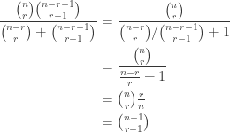
 ; note one may interpret an
  -tabloid as an ordered pair
  encoding the path of length 3 with edges
  and
and  . There is a
  acts on the set of set partitions of
  into
into  , where
  is the partition obtained from
  . So everything is in place to prove a version of the Erdős–Ko–Rado Theorem for perfect matchings. Update. I am grateful to Ehud for pointing out that this has
  . Perhaps, one day, this will be explained by defining the symmetric group as a group of automorphisms of a vector space over the field with one element. The analogue of the permutation module
  is that the maximum number of
  for
for  , where the
  -dimensional subspaces of
  . Thus the maximum is attained by taking all the subspaces containing a fixed line, in precise analogy with the case for sets. (Note also that if
  then any two
  is to
is to  where
where  is to
is to  .) Chapter 13 of his book has, I think, exactly what we need to prove the analogue of the lemma above. Update: I also just noticed that Section 8.6 of Harmonic analysis on finite groups by Ceccherini-Silberstein, Scarabotti and Tolli, titled ‘The
  where
where  is the maximal parabolic subgroup stabilising a chosen
  -dimensional subspace.
 and let
  be the permutation module of
  , let
, let  be the map sending a subspace to the formal linear combination of all
  -Specht module
  is then the intersection of the kernels of all the
  for
for  . Moreover if we set
 and
and  and
and  for
for  .
. .
. for
for  . An arbitrary
  in
in 
 and
and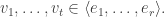
 such subspaces. Taking
  we get the result.
  when
when  and
and  when
when  by computer calculations. Note also that the
  counts, up to a power of
  , in good analogy with the symmetric group case. But it seems some careful analysis of reduced row-echelon forms (like the argument for the degree of
  .
. , and it is
 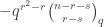 . Putting this into Hoffman’s bound and using that the subspaces graph is regular of degree
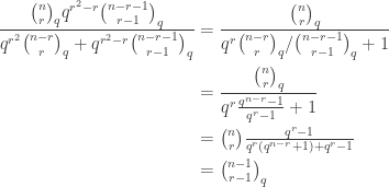
 on a vector space
  and
and  . In particular the actions of
 ,
,  and
and  be finite groups with
  . Then, for each
  , we have
 with
with  acting on the left on
  acting on the right, diagonally on each of the
  and
and  then one joint orbit is
 so we expect the stabiliser of points in the orbit to have order
  ; a little thought shows that the stabiliser of
  is
is
 : even though we are working in
  , it is not the case that the stabiliser factors as
  .
. rather than the formally correct
  .
. .
. where
where  is the subgroup of those
  fixing setwise the orbit
  . Moreover
  -modules
  .
. -modules
 as a
as a  -module in the second line and as a
  -module in the third line.
 is a normal subgroup of a permutation group
  then the orbits of
  . Then
  . This shows that
  and by symmetry equality holds.
 such that
  for some
  for some
  . These are equivalent conditions: take
  and use that the actions commute. Finally, identifying
 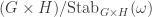 we see that
  . Since
  , as required.
 if and only if
  has a submodule isomorphic to
 ![\dim V = [K : L]\dim U](https://s0.wp.com/latex.php?latex=%5Cdim+V+%3D+%5BK+%3A+L%5D%5Cdim+U&bg=ffffff&fg=333333&s=0&c=20201002) . In this case we take
. In this case we take  -module
  .
. for induction on the left, we can state the following corollary with left- and right-actions.
 is a left
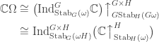
 and
and  that respect the blocks
  ,
,  ,
,  ,
,  shown by the rooted trees in the graph below. The matching
  .
.
 and both
 . This is shown graphically below.
 . On the other hand, the permutation
  cannot be undone by a permutation in
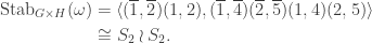
 .
.