PCA revisited: using principal components for classification of faces

This is a short post following the previous one (PCA revisited).

In this post I’m going to apply PCA to a toy problem: the classification of faces. Again I’ll be working on the Olivetti faces dataset. Please visit the previous post PCA revisited to read how to download it.

The goal of this post is to fit a simple classification model to predict, given an image, the label to which it belongs. I’m goint to fit two support vector machine models and then compare their accuracy.

The

1. The first model uses as input data the raw (scaled) pixels (all 4096 of them). Let’s call this model “the data model”.
2. The second model uses as input data only some principal components. Let’s call this model “the PCA model”.

PCA revisited

Principal component analysis (PCA) is a dimensionality reduction technique which might come handy when building a predictive model or in the exploratory phase of your data analysis. It is often the case that when it is most handy you might have forgot it exists but let’s neglect this aspect for now ;)

I decided to write this post mainly for two reasons:

1. I had to make order in my mind about the terminology used and complain about a few things.
2. I wanted to try to use PCA in a meaningful example.

Getting AI smarter with Q-learning: a simple first step in Python

Yesterday I found an “old” script I wrote during a morning in the last semester. I remember being a little bored and interested in the concept of Q-learning. That was about the time Alpha-Go had beaten the world champion of Go and by reading here and there I found out that a bit of Q-learning mixed with deep learning might have been involved.

Building a (reusable?) deep neural network model using Tensorflow

I’ve been experimenting for more than two months with Tensorflow, and while I find it a bit more “low level” if compared to other libraries for machine learning, I like it and hopefully I am getting better at using it. During the learning process I found some minor “obstacles” so I decided to write a short tutorial on how to use this amazing deep learning library.

Image recognition tutorial in R using deep convolutional neural networks (MXNet package)

This is a detailed tutorial on image recognition in R using a deep convolutional neural network provided by the MXNet package. After a short post I wrote some times ago I received a lot of requests and emails for a much more detailed explanation, therefore I decided to write this tutorial. This post will show a reproducible example on how to get 97.5% accuracy score on a faces recognition task in R.

Plain vanilla recurrent neural networks in R: waves prediction

While continuing my study of neural networks and deep learning, I inevitably meet up with recurrent neural networks.

Recurrent neural networks (RNN) are a particular kind of neural networks usually very good at predicting sequences due to their inner working. If your task is to predict a sequence or a periodic signal, then using a RNN might be a good starting point. Plain vanilla RNN work fine but they have a little problem when trying to “keep in memory” events occured, say for instance, more than 20 steps back. The solution to this problem has been addressed with the development of a model called LSTM network. As far as I know, LSTM should usually be preferred to a plain vanilla RNN when possible as it yields better results.

Image recognition in R using convolutional neural networks with the MXNet package

Among R deep learning packages, MXNet is my favourite one. Why you may ask? Well I can’t really say why this time. It feels relatively simple, maybe because at first sight its workflow looks similar to the one used by Keras, maybe because it was my first package for deep learning in R or maybe because it works very good with little effort, who knows.

MXNet is not available on CRAN but it can be easily installed either by using precompiled binaries or by building the package from scratch. I decided to install the GPU version but for some reason my GPU did not want to collaborate so I installed the CPU one that should be fine for what I plan on doing.

As a first experiment with this package, I decided to try and complete some image recognition tasks. However, the first big problem is where to find images to work on, while at the same time not using the same old boring datasets. ImageNet is the correct answer! It provides a collection of URLs to images publicly available that can be downloaded easily using a simple R or Python script.

Predicting creditability using logistic regression in R: cross validating the classifier (part 2)

Now that we fitted the classifier and run some preliminary tests, in order to get a grasp at how our model is doing when predicting creditability we need to run some cross validation methods.
Cross validation is a model evaluation method that does not use conventional fitting measures (such as R^2 of linear regression) when trying to evaluate the model. Cross validation is focused on the predictive ability of the model. The process it follows is the following: the dataset is splitted in a training and testing set, the model is trained on the testing set and tested on the test set.

Note that running this process one time gives you a somewhat unreliable estimate of the performance of your model since this estimate usually has a non-neglectable variance.

Predicting creditability using logistic regression in R (part 1)

As I said in the previous post, this summer I’ve been learning some of the most popular machine learning algorithms and trying to apply what I’ve learned to real world scenarios. The German Credit dataset provided by the UCI Machine Learning Repository is another great example of application.

The German Credit dataset contains 1000 samples of applicants asking for some kind of loan and the creditability (either good or bad)  alongside with 20 features that are believed to be relevant in predicting creditability. Some examples are: the duration of the loan, the amount, the age of the applicant, the sex, and so on. Note that the dataset contains both categorical and quantitative features.
This is a classical example of a binary classification task, where our goal is essentially to build a model that can improve the selection process of the applicants.

RandomForestClassifier on the cars dataset ML

Since the beginning of this summer I have been practicing a lot with Scikit-learn to improve my knowledge of Machine Learning both on theory and practice. Last week I also tried to tackle some of the Kaggle competitions although they are really tough if you wish to get into the top 50 best scores. Perhaps I will post something about the experience in the future.

Scikit-learn is a (almost) ready to use package for Machine Learning in Python. It is so very user friendly and in some cases not that much coding around is needed to achieve interesting results such as in the case of the cars dataset.

The cars dataset, from the UCI Machine Learning Repository, is a collection of about 1700 entries of cars each with 6 features that can be easily recognized by the name (buying, maint, doors, persons, lug_boot, safety). Check the dataset description for more detailed information. The feature to be predicted is “class” and the possible values are unacc,acc,good,v-good. Most of the features are categorical, therefore they need to be encoded into numbers. Pandas is great for quick features encoding.

Basic Hidden Markov model

A hidden Markov model is a statistical model which builds upon the concept of a Markov chain.

The idea behind the model is simple: imagine your system can be modeled as a Markov chain and the signals emitted by the system depend only on the current state of the system. If the states of the system are not visible and what you can observe are only the emitted signals, then this is a Hidden Markov model.

Simple regression models in R

Linear regression models are one the simplest and yet a very powerful models you can use in R to fit observed data and try to predict quantitative phenomena.

Say you know that a certain variable y is somewhat correlated with a certain variable x and you can reasonably get an idea of what y would be given x. A class example is the price of houses (y) and square meters (x). It is reasonable to assume that, within a certain range and given the same location, square meters are correlated with the price of the house. As a first rough approximation one could try out the hypothesis that price is directly proportional to square meters.

Now what if you would like to predict the possible price of a flat of 80 square meters? Well, an initial approach could be gathering the data of houses in the same location and with similar characteristics and then fit a model.

A linear model with one predicting variable might be the following:

Alpha and Beta can be found by looking for for the two values that minimise the error of the model relative to the observed data. Basically the procedure of finding the two coefficient is equivalent to finding the “closest” line to our data. Of course this will still be an estimate and it will probably not match any of the observed values.

How to estimate probability density function from sample data with Python

Suppose you have a sample of your data, maybe even a large sample, and you want to draw some conclusions based on its probability density function. Well, assuming the data is normally distributed, a basic thing to do is to estimate mean and standard deviation, since to fit a normal distribution those two are the only parameters you need.

However, sometimes you might not be that happy with the fitting results. That might be because your sample does not looks exactly bell shaped and you are wondering what would happened if the simulation you ran had taken this fact into account.

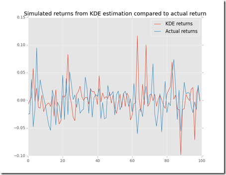
For instance, take stock returns, we know they are not normally distributed furthermore there is the “fat tails” problem to take into account. At least it would be interesting estimate a probability density function and then compare it to the parametric pdf you used before.

Here below is a simple example of how I estimated the pdf of a random variable using gaussian_kde from scipy

and here is the plot that we get

What we can see is that the estimated pdf is “more dense” around the mean and has some more density on the tails.

Let’s use this data to simulate a sample

For sure in this randomly generated sample there are some extreme values and they look close to the actual sample.

Hope this was interesting and useful.

 

---

Disclaimer
This article is for educational purpose only. The author is not responsible for any consequence or loss due to inappropriate use. The article may well contain mistakes and errors. The numbers used might not be accurate. You should never use this article for purposes different from the educational one.

Image scaling

This is a script that has been resting on my desktop for months. Basically I would like to take my knowledge of image recognition with machine learning a step further and this is a simple step towards that direction.

The basic idea behind the script is to convert the image in a 0 and 1 format which is easier to process with machine learning algorithms. After I wrote the script, I found out there is a function in sklearn that does something similar, anyway I thought I could share the piece of code I wrote, perhaps it could be useful to someone.

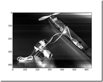
This the image I started with

By using the following script we can convert the image in a more manageable format

This is the result we obtain, A and B respectively

Only numbers between 0 and 1 are used in the picture A above while the picture below uses only 0s and 1.

For sure we loose some information, however this is just a raw script, perhaps I can do better in the future. However, this is a rather complicated image (not to mention the fact that it’s the only sample I have got) the script should yield better results with simpler images and shapes.

Handwritten number recognition with Python (Machine Learning)

Here I am again with Machine Learning! This time I’ve achieved a great result though (for me at least!). By using another great dataset from UCI I was able to write a decent ML script which scored 95% in the testing part! I am really satisfied with the result.

Here is a sample of what the script should be able to read (in the example the number 9):

Some numbers, as the one above, were clear, others not so clear, since they were handwritten and then somehow (I do not know how) converted into digital images.

I had a hard time figuring out how the attributes in the dataset were coded but in the end I managed to figure it out! I guess making up such a dataset was a really long and boring work.

Anyway here is my script and below you can find the result of the test on the last 50 numbers or so.

This time I got 89% success rate! Pretty good I guess! I wonder whether I could train Python to recognize other things, maybe faces or other! Well first of all I have to figure out how to convert a picture into readable numpy arrays. Readable for Python of course!! If you have any suggestion please do leave a comment!

Here below is the citation of the source where I found the dataset “Semeion Handwritten Digits Data Set”:

Bache, K. & Lichman, M. (2013). UCI Machine Learning Repository [http://archive.ics.uci.edu/ml]. Irvine, CA: University of California, School of Information and Computer Science.

and

Semeion Research Center of Sciences of Communication, via Sersale 117, 00128 Rome, Italy
Tattile Via Gaetano Donizetti, 1-3-5,25030 Mairano (Brescia), Italy.

 

Hope this was interesting!

Poker hands recognition (Machine Learning)

A few months ago I downloaded the scikit-learn package for Python, for those of you who might not be aware, scikit-learn is a powerful yet very simple package useful to apply machine learning. Basically they give you “all” the algorithms you may need and you “only” have to get the data and make it ready to feed into the scikit-learn algorithm.

Anyway, I only recently had time to check it out and write some code, furthermore only recently I found a great site full of sample datasets dedicated to machine learning (check it out here). Since the data from this great site is more or less in the right shape for being ready to import (.txt files or similar) the only task left to the programmer is to put it into numpy arrays.

This is one of my first attempt at generating a “real” machine learning program.

I won’t post the pre-settings script since it is pretty boring, instead I’ll briefly describe the pre-setting: basically, using a simple script I’ve splitted the training samples from the database in two .txt files trainingP.txt and target.txt respectively. TrainingP.txt contains the questions (the hands of poker) and target.txt contains the answers (=the score, that’s to say poker, full house etc… coded into numbers according to the description given in the database description file).

Below is the ml script: it is composed of 3 parts: setting, training and testing

setting: import the training sets and fit them into numpy arrays of the correct shape

training: fit the data into the model using scikit-learn

testing: test the algorithm and check what it has learned so far! Some statistics are printed, for reference. Check the results below!

So far the best score is 56.4%, I wonder if I did everything correctly! Anyway soon I will post a script with better results and achievements!

Below is the citation of the source of the database, according to their citation policy.

The name of the dataset is Poker Hand and it is from:

Bache, K. & Lichman, M. (2013). UCI Machine Learning Repository[http://archive.ics.uci.edu/ml]. Irvine, CA: University of California, School of Information and Computer Science.

Multivariable gradient descent

This article is a follow up of the following:
Gradient descent algorithm

Here below you can find the multivariable, (2 variables version) of the gradient descent algorithm. You could easily add more variables. For sake of simplicity and for making it more intuitive I decided to post the 2 variables case. In fact, it would be quite challenging to plot functions with more than 2 arguments.

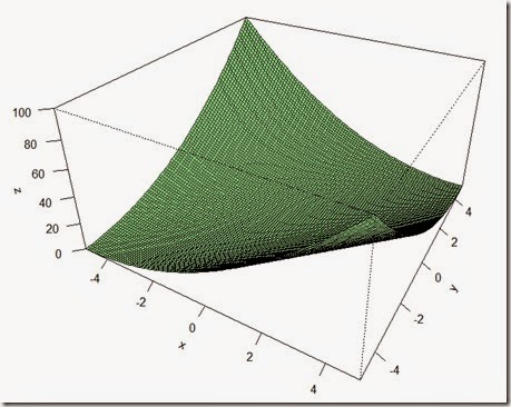
Say you have the function f(x,y) = x**2 + y**2 –2*x*y plotted below (check the bottom of the page for the code to plot the function in R):

Well in this case, we need to calculate two thetas in order to find the point (theta,theta1) such that f(theta,theta1) = minimum.

Here is the simple algorithm in Python to do this:

This function though is really well behaved, in fact, it has a minimum each time x = y. Furthermore, it has not got many different local minimum which could have been a problem. For instance, the function here below would have been harder to deal with.

Finally, note that the function I used in my example is again, convex.
For more information on gradient descent check out the wikipedia page here.
Hope this was useful and interesting.

R code to plot the function

Gradient descent algorithm

Today I’m going to post a simple Python implementation of gradient descent, a first-order optimization algorithm. In Machine Learning this technique is pretty useful to find the values of the parameters you need. To do this I will use the module sympy, but you can also do it manually, if you do not have it.

The idea behind it is pretty simple. Imagine you have a function f(x) = x^2 and you want to find the value of x, let’s call it theta, such that f(theta) is the minimum value that f can assume. By iterating the following process a sufficient number of times, you can obtain the desired value of theta:

 

Now, for this method to work, and theta to converge to a value, some conditions must be met, namely:
-The function f must be convex
-The value of alpha must not be too large or too small, since in the first case you’ll end up with the value of theta diverging and in the latter you’ll approach the desired value really slowly
-Depending on the function f, the value of alpha can change significantly.

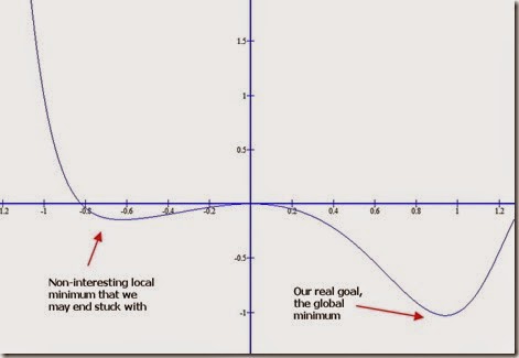
Note that, if the function has local minimums and not just an absolute minimum, this optimization algorithm may well end “trapped” in a local minimum and not find your desired global minimum. For the sake of argument, suppose the function below goes to infinity as x gets bigger and that the global minimum is somewhat near 1. With the algorithm presented here, you may well end up with x = –0.68 or something like that as an answer when you are looking roughly for x = 0.95.

In this case of course, it is trivial to find out the value and you don’t even need derivatives. However, for a different function it may not be that easy, furthermore for multivariable functions it may be even harder (in the next article I will cover multivariable functions).

Here is the Python code of my implementation of the algorithm

Hope this was interesting and useful.

A first really shy approach to Machine Learning using Python

The day before yesterday I came across Machine Learning: WOW… I got stuck at my pc for an hour wondering about and watching the real applications of this great subject.

I was getting really excited! Then, after an inspiring vide on YouTube, I decided it was time to act. My fingers wanted desperately to type some “smart” code so I decided to write a program which could  recognize the language into which a given text is written.

I do not know if this is actually a very primitive kind of Machine Learning program (I somehow doubt it) therefore I apologize to all those who know more on the subject but let me dream for now.

Remember the article on letter frequency distribution across different languages?? Back then I knew it would be useful again (although I did not know for what)!! If you would like to check it out or refresh your memory, here it is.

Name of the program: Match text to language

This simple program aims to be an algorithm able to distinguish
written text by recognizing what language a text
was written in.

The underlying hypothesis of this model are the following:
1. Each language has a given characters distribution which is different from the others. Characters distributions are generated by choosing randomly Wikipedia pages in each language.
2. Shorter sentences are more likely to contain common words that uncommon one.

The first approach to build a program able to do such a task was to build a character distribution for each of the languages used using the code in the frequency article. Next, given a string, (sentence) the program should be able to guess the language by comparing the characters distribution in the sentence with the actual distributions of the languages.

This approach, for sentences longer than 400 characters seems to work fine. However, if the sentence were to be shorter than 400 characters, a mismatch might occur. In order to avoid this, I have devised a naive approach: the shorter the sentence, the more likely the words in it are the most common. Therefore, for each language,a list of 50 most common words has been loaded and is used to double check the first guess based on the character frequency only in case the length of the sentence is less than a given number of characters (usually 400).

Note that this version of the program assumes that each language distribution has already been generated, stored in .txt format and it simply loads it from a folder. You can find and download the distributions here.

So far the program seem to work on text of different length. Here below are some results:

In these first two examples I used bigger sample sentences

In this last example, the sentence was really short, it was just 37 characters, something like: “Diese ist eine schoene Satze auf Deutsch”. In this case it was hard to draw a distribution which could match the German one. In fact the program found French and was really far away from the right answer indeed. The double-check algorithm kicked in the right answer (Lang checked).

Hope this was interesting.