Downloaded 136 times

![1
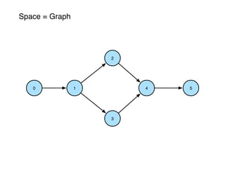
2
3
0 4 5
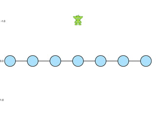
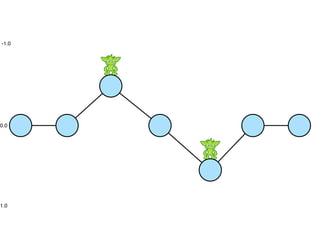
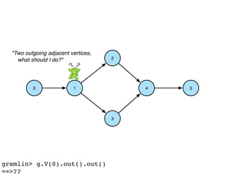
gremlin> g.V(0)
==>v[0]](https://image.slidesharecdn.com/quantum-gremlin-graphday-160114154937/85/Quantum-Processes-in-Graph-Computing-37-320.jpg)
![1
2
3
0 4 5
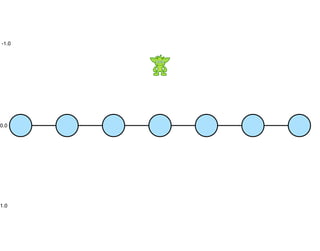
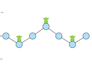
gremlin> g.V(0).out()
==>v[1]](https://image.slidesharecdn.com/quantum-gremlin-graphday-160114154937/85/Quantum-Processes-in-Graph-Computing-38-320.jpg)
![1
2
3
0 4 5
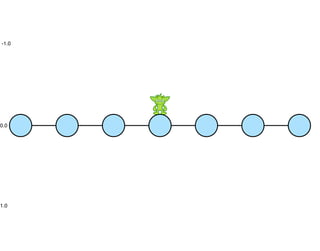
gremlin> g.V(0).out().out()
==>v[2]
==>v[3]](https://image.slidesharecdn.com/quantum-gremlin-graphday-160114154937/85/Quantum-Processes-in-Graph-Computing-40-320.jpg)
![1
2
3
0 4 5
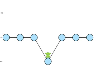
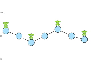
gremlin> g.V(0).out().out()
==>v[2]
==>v[3]
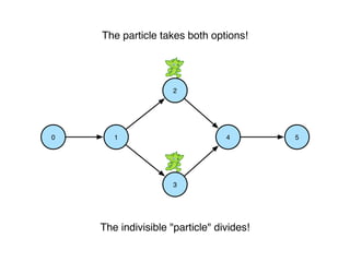
2 particles are created from 1.
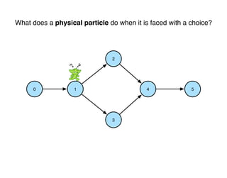
In graph computing: "There are two legal paths, so take both."
In physical computing: "Violates conservation of energy law (matter is created)."](https://image.slidesharecdn.com/quantum-gremlin-graphday-160114154937/85/Quantum-Processes-in-Graph-Computing-41-320.jpg)
![1
2
3
0 4 5
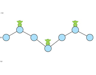
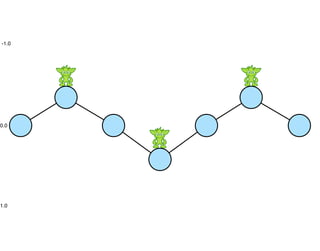
gremlin> g.V(0).out().out().out()
==>v[4]
==>v[4]
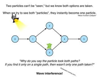
In graph computing: "Two length 3 paths lead to vertex 4."
In physical computing: "The twin particles coexist at vertex 4."](https://image.slidesharecdn.com/quantum-gremlin-graphday-160114154937/85/Quantum-Processes-in-Graph-Computing-42-320.jpg)
![1
2
3
0 4 5
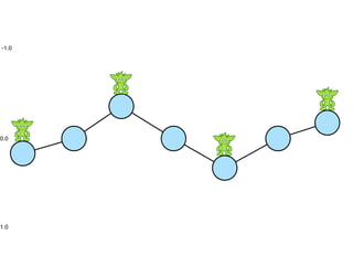
gremlin> g.V(0).out().out().out().out()
==>v[5]
==>v[5]
In graph computing: "Two length 3 paths lead to vertex 5."
In physical computing: "The twin particles coexist at vertex 5."](https://image.slidesharecdn.com/quantum-gremlin-graphday-160114154937/85/Quantum-Processes-in-Graph-Computing-43-320.jpg)
![Classical Initial Step
The particle has a definite location and a spin/potential to the left.
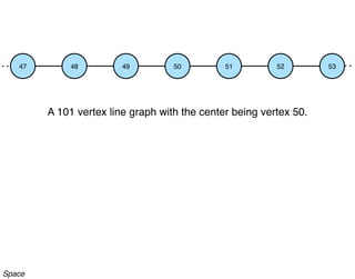
48 49 5047 51 52 53
[1, 0]
[1,0]50
left-ness
right-ness
For each option (degree of freedom),
we need a vector component.
In the article, we call it "traversal superposition."](https://image.slidesharecdn.com/quantum-gremlin-graphday-160114154937/85/Quantum-Processes-in-Graph-Computing-52-320.jpg)
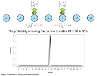
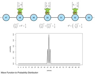
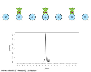
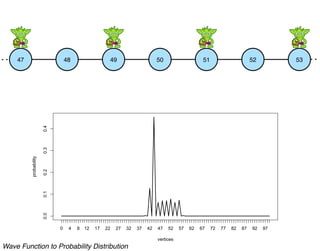
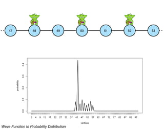
![0.00.20.40.60.81.0
vertices
probability
0 4 8 12 17 22 27 32 37 42 47 52 57 62 67 72 77 82 87 92 97
48 49 5047 51 52 53
The probability of seeing the particle at vertex 50 is 100%.
[1, 0]
12
+ 02
= 1
Wave Function to Probability Distribution](https://image.slidesharecdn.com/quantum-gremlin-graphday-160114154937/85/Quantum-Processes-in-Graph-Computing-53-320.jpg)
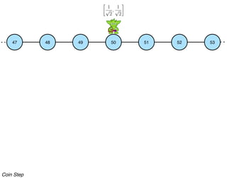
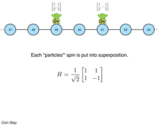
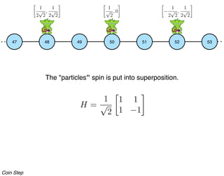
![Coin Step
48 49 5047 51 52 53
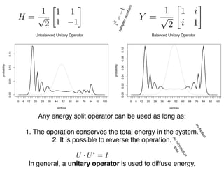
H =
1
√
2
1 1
1 −1
The particle's spin is put into superposition.
[1, 0] →
1
√
2
,
1
√
2
Ithastheoptiontogo
leftorrightsoitgoesboth!](https://image.slidesharecdn.com/quantum-gremlin-graphday-160114154937/85/Quantum-Processes-in-Graph-Computing-54-320.jpg)
![Coin Step
48 49 5047 51 52 53
H =
1
√
2
1 1
1 −1
The particle's spin is put into superposition.
[1, 0] →
1
√
2
,
1
√
2
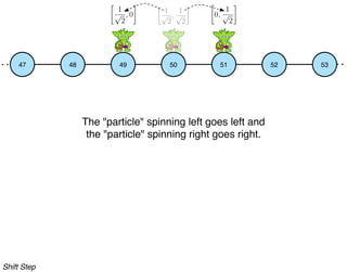
"right particles" going right flip their sign.
"left particles" going left or right keep their sign.](https://image.slidesharecdn.com/quantum-gremlin-graphday-160114154937/85/Quantum-Processes-in-Graph-Computing-55-320.jpg)
![Coin Step
48 49 5047 51 52 53
H =
1
√
2
1 1
1 −1
The particle's spin is put into superposition.
[1, 0] →
1
√
2
,
1
√
2
1
√
2
1 1
1 −1
· [1, 0] =
1√
2
1√
2
1√
2
− 1√
2
· [1, 0] =
1
√
2
,
1
√
2](https://image.slidesharecdn.com/quantum-gremlin-graphday-160114154937/85/Quantum-Processes-in-Graph-Computing-56-320.jpg)
![Coin Step
48 49 5047 51 52 53
H =
1
√
2
1 1
1 −1
The particle's spin is put into superposition.
1 ·
1
√
2
+ 0 ·
1
√
2
, 1 ·
1
√
2
+ 0 · −
1
√
2
=
1
√
2
,
1
√
2
[1, 0] →
1
√
2
,
1
√
2
1
√
2
1 1
1 −1
· [1, 0] =
1√
2
1√
2
1√
2
− 1√
2
· [1, 0] =
1
√
2
,
1
√
2](https://image.slidesharecdn.com/quantum-gremlin-graphday-160114154937/85/Quantum-Processes-in-Graph-Computing-57-320.jpg)
![Classical Particle
13 14 1512 16 17 18
[1, 0]
0.00.20.40.60.81.0
vertices
probability
0 4 8 12 17 22 27 32 37 42 47 52 57 62 67 72 77 82 87 92 97](https://image.slidesharecdn.com/quantum-gremlin-graphday-160114154937/85/Quantum-Processes-in-Graph-Computing-86-320.jpg)
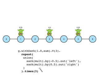
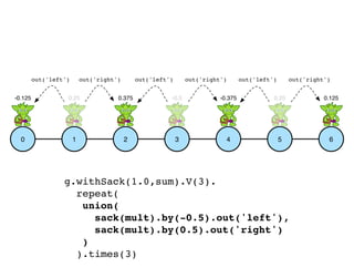
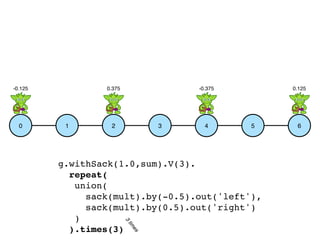
![g.withSack([1,0],sackSum).V(50).
repeat(
sack(hadamard).
union(
sack(project).by(constant([1,0])).out('left'),
sack(project).by(constant([0,1])).out('right')
)
).times(50).
group().by(id).by(sack().map(norm)).
unfold().sample(1).by(values)
48 49 5047 51 52 53](https://image.slidesharecdn.com/quantum-gremlin-graphday-160114154937/85/Quantum-Processes-in-Graph-Computing-89-320.jpg)
![48 49 5047 51 52 53
[1, 0]
g.withSack([1,0],sackSum).V(50).
repeat(
sack(hadamard).
union(
sack(project).by(constant([1,0])).out('left'),
sack(project).by(constant([0,1])).out('right')
)
).times(50).
group().by(id).by(sack().map(norm)).
unfold().sample(1).by(values)
Classical Initial Step
sackSum = { a,b -> [a[0] + b[0],a[1] + b[1]] }](https://image.slidesharecdn.com/quantum-gremlin-graphday-160114154937/85/Quantum-Processes-in-Graph-Computing-90-320.jpg)
![hadamard = { a,b ->
[(1/Math.sqrt(2)) * (a[0] + a[1]), (1/Math.sqrt(2)) * (a[0] - a[1])]
}
g.withSack([1,0],sackSum).V(50).
repeat(
sack(hadamard).
union(
sack(project).by(constant([1,0])).out('left'),
sack(project).by(constant([0,1])).out('right')
)
).times(50).
group().by(id).by(sack().map(norm)).
unfold().sample(1).by(values)
Coin Step
H =
1
√
2
1 1
1 −1
48 49 5047 51 52 53
1
√
2
,
1
√
2](https://image.slidesharecdn.com/quantum-gremlin-graphday-160114154937/85/Quantum-Processes-in-Graph-Computing-91-320.jpg)
![project = { a,b -> [a[0] * b[0], a[1] * b[1]] }
g.withSack([1,0],sackSum).V(50).
repeat(
sack(hadamard).
union(
sack(project).by(constant([1,0])).out('left'),
sack(project).by(constant([0,1])).out('right')
)
).times(50).
group().by(id).by(sack().map(norm)).
unfold().sample(1).by(values)
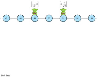
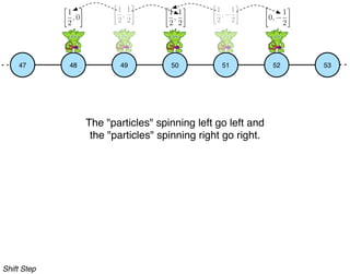
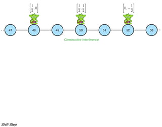
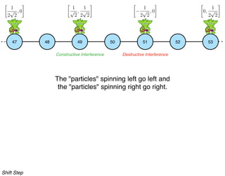
Shift Step
48 49 5047 51 52 53
1
√
2
, 0 0,
1
√
2
1
√
2
,
1
√
2](https://image.slidesharecdn.com/quantum-gremlin-graphday-160114154937/85/Quantum-Processes-in-Graph-Computing-92-320.jpg)
![g.withSack([1,0],sackSum).V(50).
repeat(
sack(hadamard).
union(
sack(project).by(constant([1,0])).out('left'),
sack(project).by(constant([0,1])).out('right')
)
).times(50).
group().by(id).by(sack().map(norm)).
unfold().sample(1).by(values)
Diffuse the wave function for 50 steps
48 49 5047 51 52 53](https://image.slidesharecdn.com/quantum-gremlin-graphday-160114154937/85/Quantum-Processes-in-Graph-Computing-93-320.jpg)
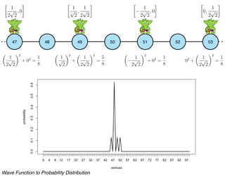
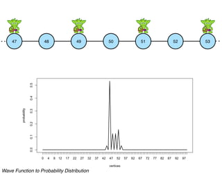
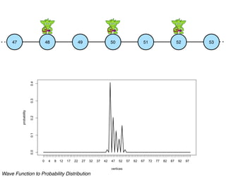
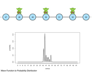
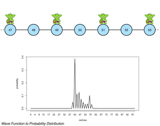
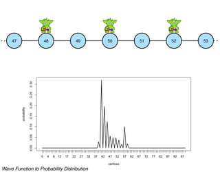
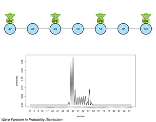
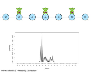
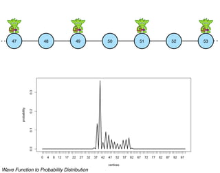
![0.000.050.100.15
vertices
probability
0 4 8 12 17 22 27 32 37 42 47 52 57 62 67 72 77 82 87 92 97
norm = { Math.pow(it.get()[0],2) +
Math.pow(it.get()[1],2) }
g.withSack([1,0],sackSum).V(50).
repeat(
sack(hadamard).
union(
sack(project).by(constant([1,0])).out('left'),
sack(project).by(constant([0,1])).out('right')
)
).times(50).
group().by(id).by(sack().map(norm)).
unfold().sample(1).by(values)
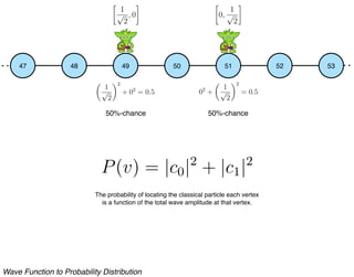
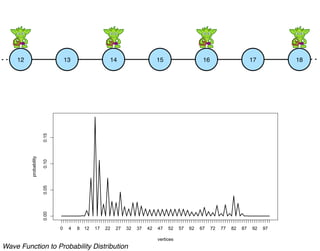
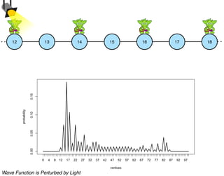
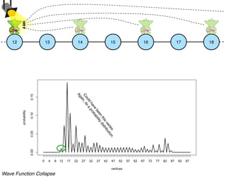
Wave Function to Probability Distribution
13 14 1512 16 17 18
P(v) = |c0|2
+ |c1|2](https://image.slidesharecdn.com/quantum-gremlin-graphday-160114154937/85/Quantum-Processes-in-Graph-Computing-94-320.jpg)
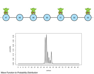
![g.withSack([1,0],sackSum).V(50).
repeat(
sack(hadamard).
union(
sack(project).by(constant([1,0])).out('left'),
sack(project).by(constant([0,1])).out('right')
)
).times(50).
group().by(id).by(sack().map(norm)).
unfold().sample(1).by(values)
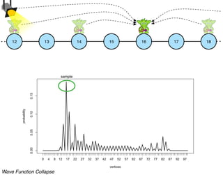
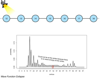
Wave Function Collapse (Classical Particle Manifested)
13 14 1512 16 17 18
0.000.050.100.15
vertices
probability
0 4 8 12 17 22 27 32 37 42 47 52 57 62 67 72 77 82 87 92 97
sample](https://image.slidesharecdn.com/quantum-gremlin-graphday-160114154937/85/Quantum-Processes-in-Graph-Computing-95-320.jpg)
![g.withSack([1,0],sackSum).V(50).
repeat(
sack(hadamard).
union(
sack(project).by(constant([1,0])).out('left'),
sack(project).by(constant([0,1])).out('right')
)
).times(50).
group().by(id).by(sack().map(norm)).
unfold().sample(1).by(values)
A Quantum Walk on a Line with Gremlin](https://image.slidesharecdn.com/quantum-gremlin-graphday-160114154937/85/Quantum-Processes-in-Graph-Computing-96-320.jpg)
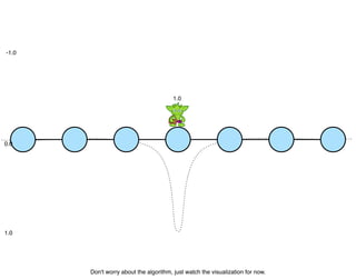
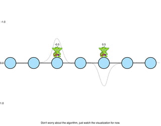
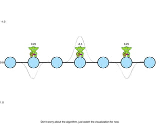
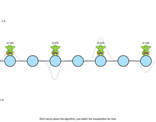
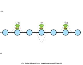
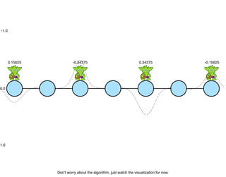
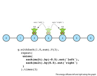
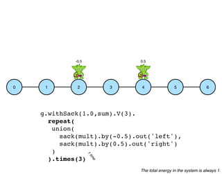
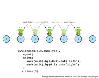
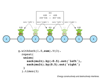
The document discusses quantum processes in graph computing, particularly focusing on the concept of energy diffusion within graph structures and its representation using Gremlin sacks. It explains how energy behaves like a wave and can undergo constructive and destructive interference when traversers split and merge. Furthermore, it relates this to quantum mechanics and the Copenhagen interpretation, illustrating how particles take multiple paths simultaneously and the behavior of wave functions.