Main features#

These features can be seen in the basic tutorial.

Open#

The reader singleton is your unique entry. It will create for you the product object corresponding to your satellite data.

You can load products from the cloud, see this tutorial. S3 and S3 Compatible Storage are working and maybe Google and Azure if rasterio supports it, but they have not been tested.

import os
from reader import Reader

# Path to your satellite data, i.e. Sentinel-2
# You can directly work with archived S2 data
path = r'S2A_MSIL1C_20200824T110631_N0209_R137_T30TTK_20200824T150432.zip'

# Path to your output directory (if not set, it will work in a temp directory)
output = os.path.abspath('.')

# Create the reader singleton
reader = Reader()
prod = reader.open(path, output_path=output, remove_tmp=True)
# remove_tmp allows you to automatically delete processing files 
# such as cleaned or orthorectified bands when the product is deleted
# False by default to speed up the computation if you want to use the same product in several part of your code

# NOTE: you can set the output directory after the creation, that allows you to use the product condensed name
# It will automatically create the output directory if needed
prod.output = os.path.join(output, prod.condensed_name)

The goal of this library is to manage only one satellite product at a time. To handle more complicated sets of products (such as mosaics, pairs or time series), please consider using EOSets.

This feature can also be used as a context manager:

import os
from reader import Reader

# Path to your satellite data, i.e. Sentinel-2
path = r'S2A_MSIL1C_20200824T110631_N0209_R137_T30TTK_20200824T150432.zip'

with Reader().open(path, remove_tmp=True) as prod:
    prod.output = os.path.join(output, prod.condensed_name)
    # Here you have access to all the temporary files

# Here not

Condensed name#

If you chose to create the output folder after creation of the Product object, you can leverage the condensed_name to name it.

The condensed_name of your product is a powerful feature: it is the more compact name possible to identify your product in a unique way, with a pattern common to every EOReader product.
It is very convenient to name in the same way all your results, to be able to sort them by date, sensors, etc.

It is constructed this way: {date}_{constellation}_{other_identifiers} (tiles, ID, instrument, etc. depending on the sensor type)

Hereunder is an example of a folder containing results for a lot of different sensors. The results are named after the condensed names, so they are easily sortable by date and sensor (here the most recent product is first).

Example of condensed names

├── DATA
│   ├── 20250128T184154_UMBRA_VV_SP_GEC
│   ├── 20241008T091030_WVLG_Standard_Multi_050246698010
│   ├── 20231031T064451_S2_T39KZU_L2A_073602
│   ├── 20231027T163107_S1_VV_VH_IW_RTC
│   ├── 20221127T214948_HLS_S30_T60FXK
│   ├── 20220828T055634_L9_152041_OLI_TIRS
│   ├── 20220828T055634_HLS_L30_T42RVR
│   ├── 20220617T042706_L7_152041_ETM
│   ├── 20220303T123054_SKY_ORTHO_PSH_u0001
│   ├── 20220118T215211_PNEO_ORT_PMS_000007338
│   ├── 20220111T222049_VIS1_PRJ_MS4_S121952
│   ├── 20210926T061012_CAPELLA_HH_SS_GEC
│   ├── 20210906T180801_RCM_HH_HV_3M_GRD
│   ├── 20210827T162210_ICEYE_VV_SC_GRD
│   ├── 20210628T054829_CSG_HH_PP_SCS
│   ├── 20210422T104727_S2THEIA_T32ULU_L2A
│   ├── 20201223T220311_SKY_ORTHO_PSH_u0002
│   ├── 20201220T104856_L8_200030_OLI_TIRS
│   ├── 20201029T105210_VENUS_SUDOUE-1_L2A
│   ├── 20201008T224018_CSK_HH_HI_DGM
│   ├── 20201005T102800_GE01_Ortho_BGRN_013187549010
│   ├── 20200926T100102_PLA_L3B
│   ├── 20200607T080134_SV1_L1B_PMS_0001022989
│   ├── 20200605T042203_TSX_HH_SM_MGD
│   ├── 20200511T023158_PLD_ORT_PMS_5547047101
│   ├── 20191215T105023_S3_OLCI_EFR
│   ├── 20191215T060906_S1_VV_VH_IW_GRD
│   ├── 20191204T101938_SAOCOM_VV_HH_VH_HV_TN_L1A
│   ├── 20191115T233722_S3_SLSTR_RBT
│   ├── 20191017T080142_RE_L3A_3754903
│   ├── 20181218T093848_SPOT6_ORT_PMS_3726409101
│   ├── 20161107T013821_GS2_L1C_MS4_12927
│   ├── 20160604T175322_RS2_HH_U_SGF
│   ├── 20160502T131229_WV03_Standard_Multi_055670633040
│   ├── 20160215T025702_SPOT7_SEN_MS_1671661101
│   ├── 20141115T055250_TDX_HH_SM_MGD
│   ├── 20121230T102407_L5_200030_MSS
│   ├── 20111112T165942_L5_029031_TM
│   ├── 20100226T032514_SPOT5_L1A_J
│   ├── 20060213T030050_SPOT4_L1A_MI
│   ├── 19930710T155617_L4_024031_TM
│   ├── 19820906T164709_L3_033028_MSS
│   ├── 19820202T155126_L2_024030_MSS
│   ├── 19771229T152402_L1_034032_MSS

Recognized paths#

EOReader always uses the directory containing the product files. Hereunder are the paths meant to be given to the reader.

Optical#

Sensor group	Folder to link
`Sentinel-2 and 3`	Main directory, `.SAFE`, `.SEN3` or `.zip`, i.e. `S2A_MSIL1C_20200824T110631_N0209_R137_T30TTK_20200824T150432.SAFE`
`Sentinel-2 Theia and Venµs`	Main directory containing the `.tif` images, i.e. `SENTINEL2A_20190625-105728-756_L2A_T31UEQ_C_V2-2`
`Landsats`	Main directory extracted or archived if Collection 2 (`.tar`), i.e. `LC08_L1TP_200030_20201220_20210310_02_T1.tar`
`Harmonized Landsat-Sentinel`	Main directory containing the `.tif` images, i.e. `HLS.S30.T42RUS.2022241T060629.v2.0`
`PlanetScope`, `SkySat` and `RapidEye`	Directory containing the `manifest.json` file, i.e. `20210406_015904_37_2407`
`DIMAP` (Pleiades, SPOTs, Vision-1, …)	Directory containing the `.JP2` files, i.e. `IMG_PHR1B_PMS_001`
`Vantor` (WorldViews, GeoEye…)	Directory containing the `.TIL` file, i.e. `013187549010_01_P001_PSH`
`SuperView-1`	Directory containing the `.shp` file, i.e. `0032100150001_01`
`GEOSAT-2`	Directory containing the `.dim` file, i.e. `DE2_PM4_L1C_000000_20161107T013821_20161107T013826_DE2_12927_DE02`
`Aleph-1` `(Satellogic)`	Directory containing the `TOA.vrt` file, i.e. `20240321_185542_636_SN43_L1D_MS_203088`

SAR#

Sensor group	Folder to link
`Sentinel-1` `RADARSAT-Constellation`	SAFE directory containing the `manifest.safe` file, i.e. `S1A_IW_GRDH_1SDV_20191215T060906_20191215T060931_030355_0378F7_3696.SAFE`
`COSMO-Skymed` 1st and 2nd Gen	Directory containing the `.h5` image, i.e. `1011117-766193`
`RADARSAT-2`	Main directory containing the `.tif` image, i.e. `RS2_OK73950_PK661843_DK590667_U25W2_20160228_112418_HH_SGF.zip`
`TerraSAR-X` `TanDEM-X` `PAZ SAR`	Directory containing the `IMAGEDATA` directory, i.e. `TDX1_SAR__MGD_SE___SM_S_SRA_20201016T231611_20201016T231616`
`ICEYE`	Directory containing the `.tif` file, i.e. `SC_124020`
`SAOCOM`	Directory containing the `.xemt` AND the `.zip` files, i.e. `11245-EOL1CSARSAO1A198523`
`CAPELLA`	Directory containing the `.tif` file, i.e. `CAPELLA_C05_SP_SLC_HH_20220320114010_20220320114013`
`UMBRA`	Directory containing the `.tif` file, i.e. `2023-11-10-09-37-28_UMBRA-04`

For example, if you want to link the following Pleiades:

├── /home/data
│   ├── DATA
│   │   ├── Call925
│   │   │   ├── 6650951101
│   │   │   │   ├── IMG_PHR1A_PMS_001
│   │   │   │   │   ├── DIM_PHR1A_PMS_202302251324499_ORT_6650951101.XML
│   │   │   │   │   ├── IMG_PHR1A_PMS_202302251324499_ORT_6650951101_R1C1.JP2
│   │   │   │   │   ├── PREVIEW_PHR1A_PMS_202302251324499_ORT_6650951101.KMZ
│   │   │   │   │   ├── ...

The product is the folder containing the DIMAP file, i.e. IMG_PHR1A_PMS_001, so the path to give to EOReader is /home/data/DATA/Call925/6650951101/IMG_PHR1A_PMS_001

Load#

load is the function for accessing product-related bands. It can load satellite bands, index, DEM bands and cloud bands according to this workflow:

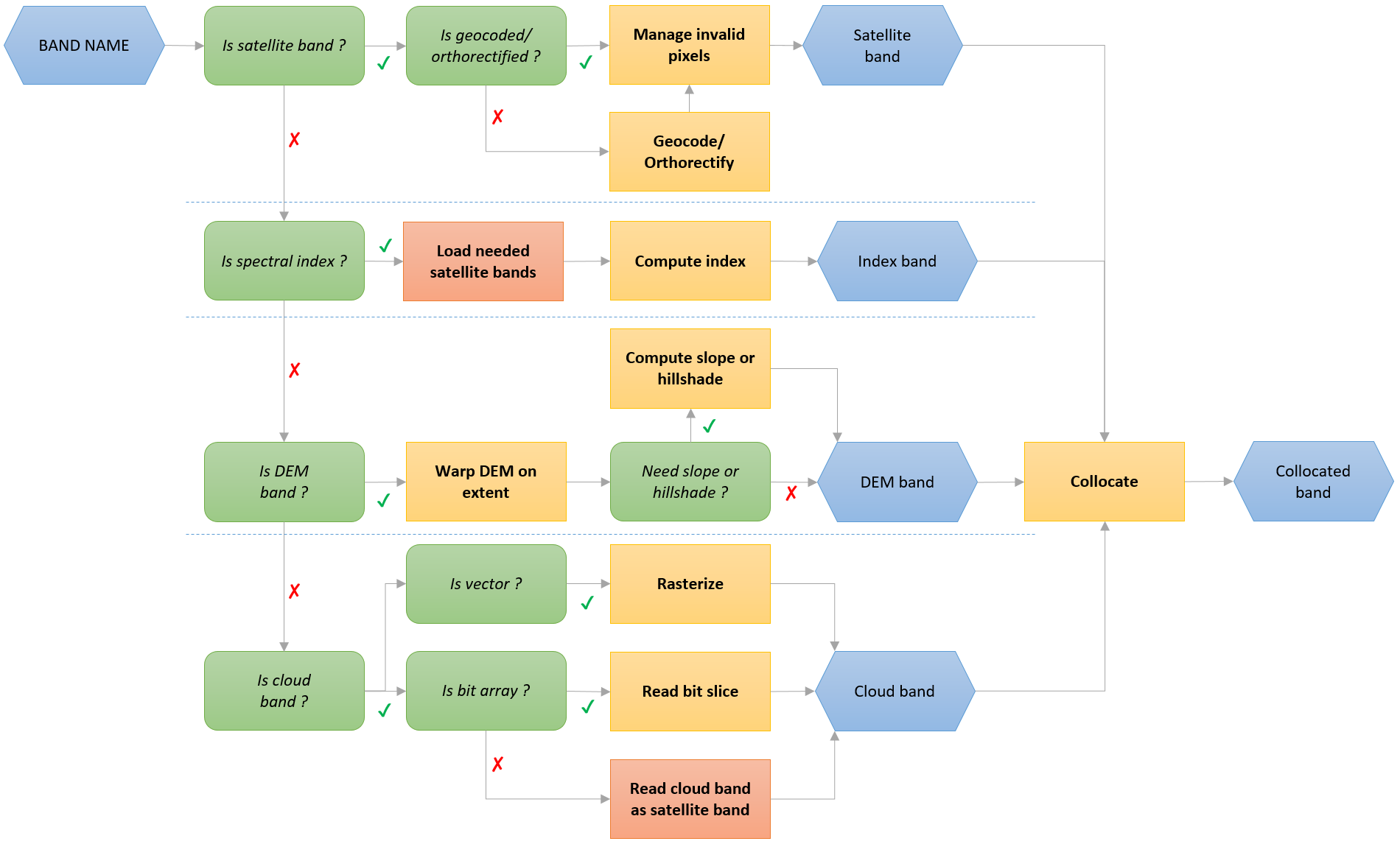
Bands can be called with their name, ID or mapped name. For example, for Sentinel-3 OLCI you can use 7, Oa07 or YELLOW. For Landsat-8, you can use BLUE or 2.

Note

For now, EOReader always loads bands with projected CRS (in UTM).

We know that this policy may be an issue for:

Sentinel-3 data that are vast and may have inaccurate georeferencing.
DIMAP data provided in WGS84 that need reprojection (and therefore time-consuming processes)

If needed, we could change in the future this to allow custom CRS. If so, do not hesitate to add comments in this issue on GitHub!

import os
from eoreader.reader import Reader
from eoreader.bands import *
from eoreader.env_vars import DEM_PATH

path = r"S2B_MSIL1C_20210517T103619_N7990_R008_T30QVE_20210929T075738.SAFE"
output = os.path.abspath("./output")
# WARNING: you can leave the output_path empty, but EOReader will create a temporary output directory,
# and you won't be able to retrieve what's has been written on disk
prod = Reader().open(path, output_path=output)

# Specify a DEM to load DEM bands
os.environ[DEM_PATH] = r"my_dem.tif"

# Get the wanted bands and check if the product can produce them
band_list = [GREEN, NDVI, TIR_1, SHADOWS, HILLSHADE]
ok_bands = to_str([band for band in band_list if prod.has_band(band)])
# [GREEN, NDVI, HILLSHADE]
# Sentinel-2 cannot produce satellite band TIR_1 and cloud band SHADOWS

# Load bands
# if pixel_size is not specified -> load at default pixel_size (10.0 m for S2 data)
bands = prod.load(ok_bands, pixel_size=20.)
# NOTE: every array that comes out `load` are collocated, which isn't the case if you load arrays separately
# (important for DEM data as they may have different grids)

Note

Index and bands are opened as xarrays with rioxarray, in float with the nodata set to np.nan. The nodata written back on disk is by convention:

-9999 for optical bands (saved in float32)
65535 for optical bands (saved in uint16)
0 for SAR bands (saved in float32), to be compliant with SNAP default nodata
255 for masks (saved in uint8)

For optical bands, only the pixels outside of the detector are set to nodata by default but this can be changed according to the user’s needs (see below).

Some additional arguments can be passed to this function, please see keywords for the list.

Methods to clean optical bands are best described here,
Sentinel-3 additional keywords use is highlighted in the corresponding notebook.
Windows can be passed to the load and stack functions (notebook).
Exogenous data can be passed to the load and stack functions (notebook).

💡 The bands will be opened with a chunk of [1, TILE_SIZE, TILE_SIZE] with TILE_SIZE coming from the EOREADER_TILE_SIZE environment variable. The TILE_SIZE default value is 2048.

💡 By default the band will be resampled following a bilinear resampling. To override this behaviour, modify the EOREADER_BAND_RESAMPLING environment variable. Note that for discrete files such as masks, the nearest resampling is set in stone.

Available values (use the number and see rasterio’s Resampling for more details and limitations):

nearest = 0
bilinear = 1
cubic = 2
cubic_spline = 3
lanczos = 4
average = 5
mode = 6
gauss = 7
max = 8
min = 9
med = 10
q1 = 11
q3 = 12
sum = 13
rms = 14

Stack#

stack is the function stacking all possible bands. It is based on the load function and then just stacks the bands and write it on disk if needed.

The bands are ordered as asked in the stack. However, they cannot be duplicated (the stack cannot contain 2 RED bands for instance)! If the same band is asked several times, its order will be the one of the last demand.

# Create a stack with the previous OK bands
stack = prod.stack(
  ok_bands,
  pixel_size=300.,
  stack_path=os.path.join(prod.output, "stack.tif")
)

Bands can be called with their name, ID or mapped name. For example, for Sentinel-3 OLCI you can use 7, Oa07 or YELLOW. For Landsat-8, you can use BLUE or 2.

Some additional arguments can be passed to this function, please see keywords for the list.

Methods to clean optical bands are best described here,
Sentinel-3 additional keywords use is highlighted in the corresponding notebook.
Windows can be passed to the load and stack functions (notebook).

Read Metadata#

EOReader gives you the access to the metadata of your product as a lxml.etree._Element followed by the namespace you may need to read them

# Access the raw metadata as an lxml.etree._Element and its namespaces as a dict:
mtd, nmsp = prod.read_mtd()

# You can access a field like that: 
datastrip_id = mtd.findtext(".//DATASTRIP_ID")
# 'S2B_OPER_MSI_L1C_DS_VGSR_20210929T075738_S20210517T104617_N79.90'

# Pay attention, for some products you will need a namespace, i.e. for planet data:
# name = mtd.findtext(f".//{nsmap['eop']}identifier")

Note

Landsat Collection 1 have no metadata with XML format, so the XML is simulated from the text file.

Note

Sentinel-3 constellations have no metadata file but have global attributes repeated in every NetCDF files. This is what you will have when calling this function:

absolute_orbit_number
comment
contact
creation_time
history
institution
netCDF_version
product_name
references
resolution
source
start_offset
start_time
stop_time
title
ac_subsampling_factor (OLCI only)
al_subsampling_factor (OLCI only)
track_offset (SLSTR only)

Plot#

If a quicklook exists, the user can plot the product. Always existing for VHR and SAR data, more rarely for other optical constellations. See Optical and SAR tutorials for examples.

# Plot product
prod.plot()

Other features#

CRS#

Get the product CRS, always in UTM.

# Product CRS (always in UTM)
prod.crs()
# CRS.from_epsg(32630)

Extent and footprint#

Get the product extent and footprint, always in UTM as a gpd.GeoDataFrame.

# Full extent of the bands as a geopandas GeoDataFrame
prod.extent()
#                                            geometry
#0   POLYGON((309780.000 4390200.000, 309780.000 4...

# Footprint: extent of the useful pixels (minus nodata) as a geopandas GeoDataFrame
prod.footprint()
#                                            geometry
#0 POLYGON Z((199980.000 4390200.000 0.000, 1999...

Please note the difference between footprint and extent:

Without nodata	With nodata

Solar angles#

Get optical product azimuth (between [0, 360] degrees) and zenith solar angles, useful for computing the Hillshade for example.

# Get azimuth and zenith solar angles
prod.get_mean_sun_angles()
# (81.0906721240477, 17.5902388851456)

Cloud Cover#

Get optical product cloud cover as specified in the metadata

# Get cloud cover
prod.get_cloud_cover()
# 0.155752635193646

Orbit direction#

Get product optical direction (useful especially for SAR data), as a OrbitDirection (ASCENDING or DESCENDING). Always specified in the metadata for SAR constellations, set to DESCENDING by default for optical data if not existing.

# Get orbit direction
prod.get_orbit_direction()
# <OrbitDirection.DESCENDING: 'DESCENDING'>

STAC#

EOReader can help you create SpatioTemporal Asset Catalog (STAC) items from every supported products, included custom ones. Those items are ready to be added in any STAC catalogue or collection. See STAC Notebook to learn more about this feature.

# Get STAC object
prod.stac

# Create STAC item
prod.stac.create_item()
# <Item id = 20210517T103619_S2_T30QVE_L1C_075738>

Some functions have different names between EOReader and STAC vocabulary. For legacy purpose, this has not been changed. Hereunder is the mapping:

prod.stac.bbox is equivalent to prod.extent but in WGS84 (EPSG:4326)
prod.stac.proj.bbox is equivalent to prod.extent
prod.stac.geometry is equivalent to prod.footprint but in WGS84 (EPSG:4326)
prod.stac.proj.geometry is equivalent to prod.footprint

Main features

Contents

Main features#

Open#

Condensed name#

Recognized paths#

Optical#

SAR#

Load#

Stack#

Read Metadata#

Plot#

Other features#

CRS#

Extent and footprint#

Solar angles#

Cloud Cover#

Orbit direction#

STAC#