Resource retrieval
Get the pre-trained net:
Basic usage
Classify an image:
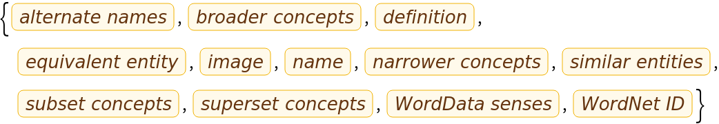
The prediction is an Entity object, which can be queried:
Get a list of available properties of the predicted Entity:
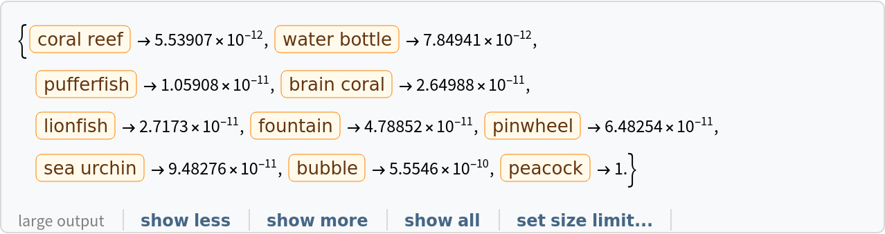
Obtain the probabilities of the ten most likely entities predicted by the net:
An object outside the list of the ImageNet classes will be misidentified:
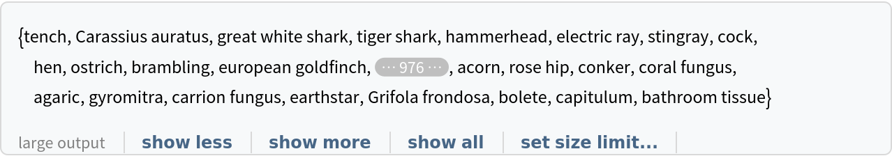
Obtain the list of names of all available classes:
Feature extraction
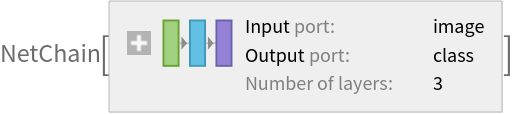
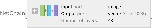
Remove the last three layers of the trained net, so that the net produces a vector representation of an image:
Get a set of images:
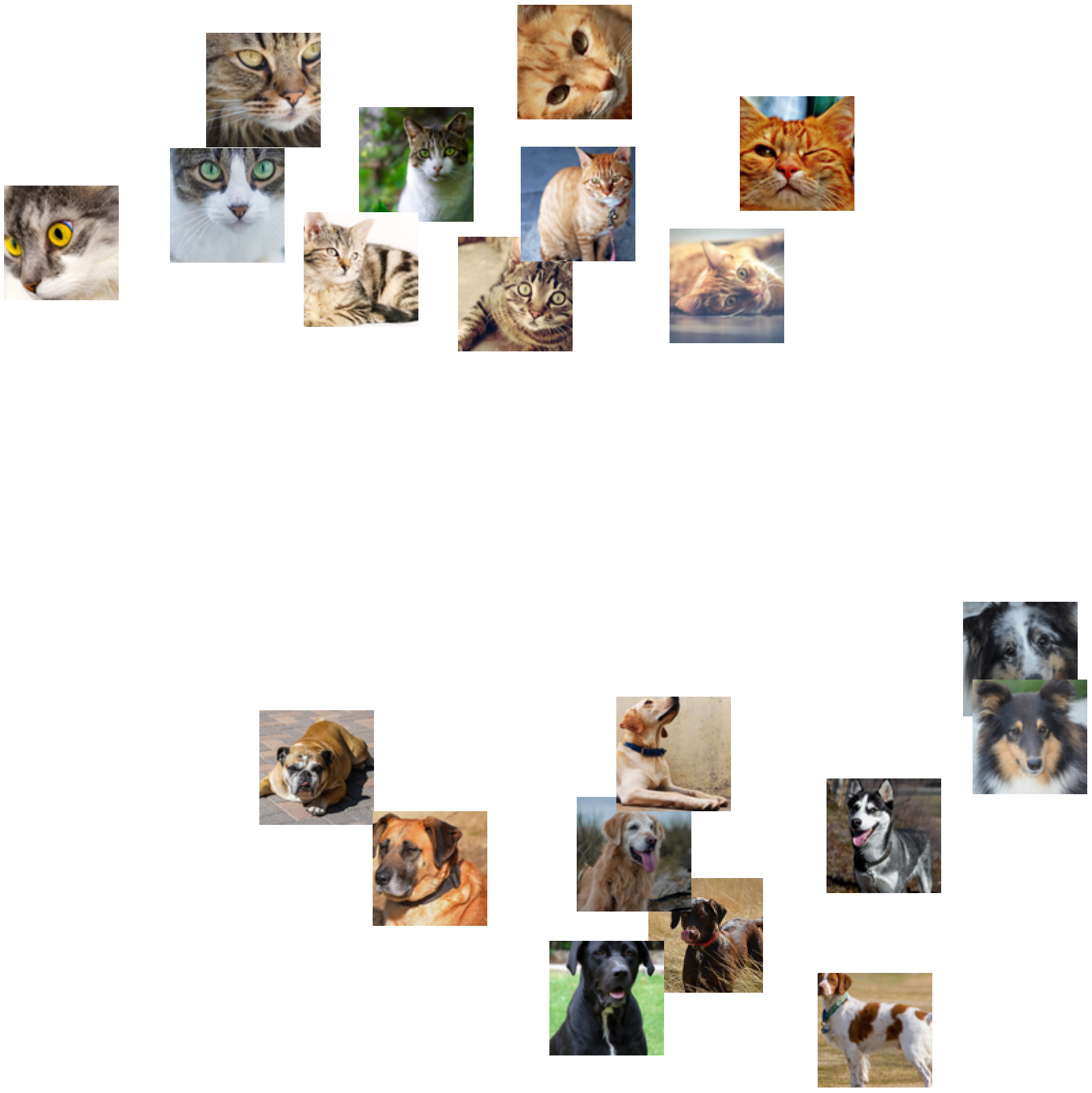
Visualize the features of a set of images:
Visualize convolutional weights
Extract the weights of the first convolutional layer in the trained net:
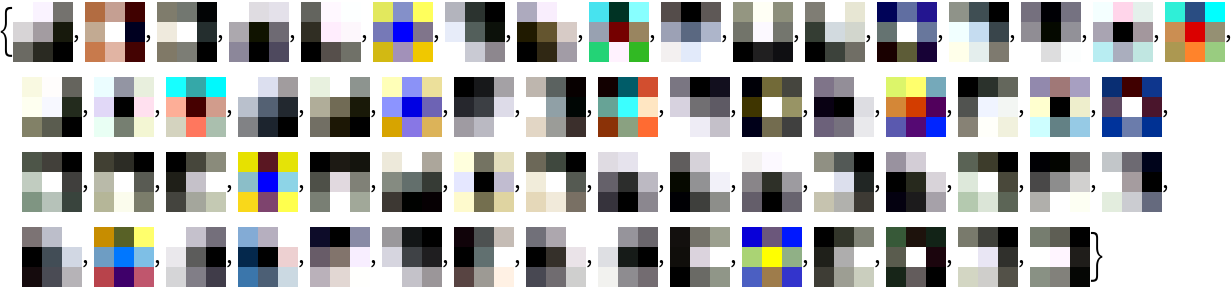
Visualize the weights as a list of 64 images of size 3x3:
Transfer learning
Use the pre-trained model to build a classifier for telling apart images of dogs and cats. Create a test set and a training set:
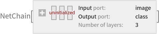
Remove the linear layer from the pre-trained net:
Create a new net composed of the pre-trained net followed by a linear layer and a softmax layer:
Train on the dataset, freezing all the weights except for those in the "linearNew" layer (use TargetDevice -> "GPU" for training on a GPU):
Perfect accuracy is obtained on the test set:
Net information
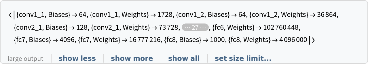
Inspect the number of parameters of all arrays in the net:
Obtain the total number of parameters:
Obtain the layer type counts:
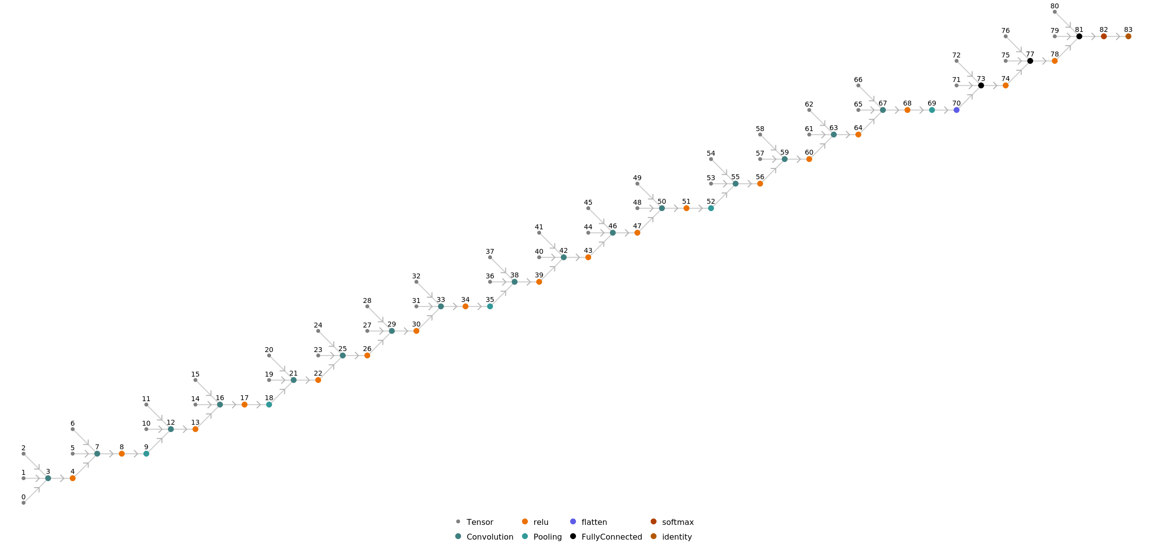
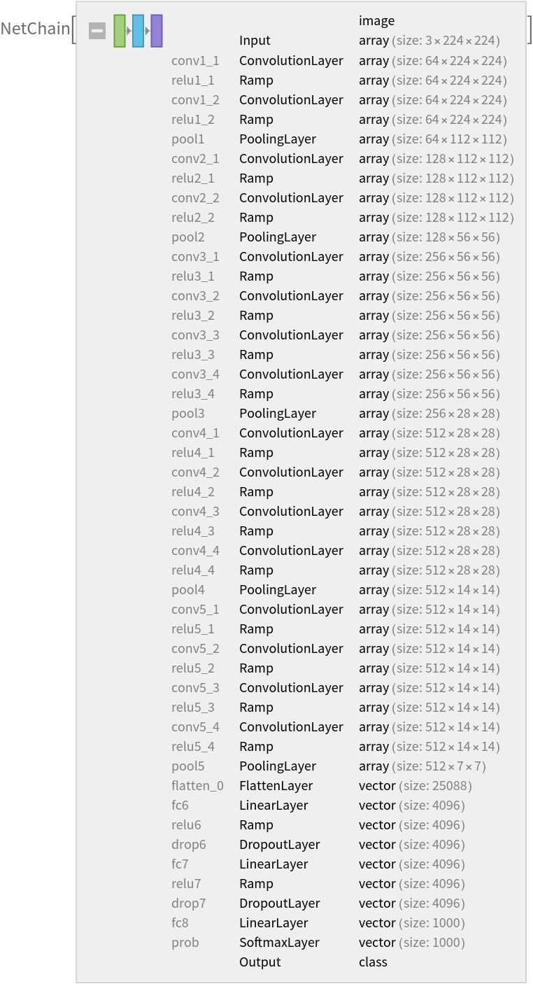
Display the summary graphic:
Export to MXNet
Export the net into a format that can be opened in MXNet:
Export also creates a net.params file containing parameters:
Get the size of the parameter file:
The size is similar to the byte count of the resource object:
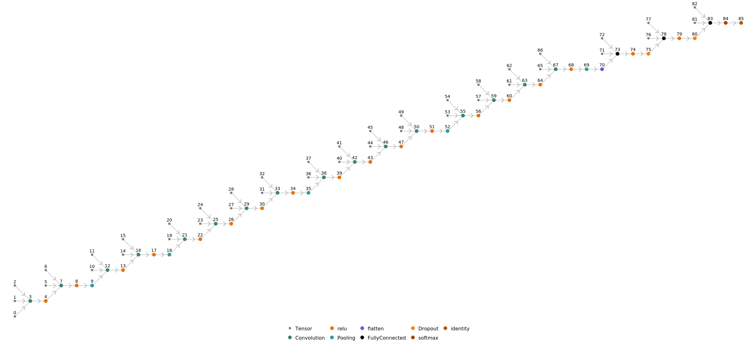
Represent the MXNet net as a graph:
![(* Evaluate this cell to get the example input *) CloudGet["https://www.wolframcloud.com/obj/364521e5-2245-4bc4-a8b0-f19cb8b761b7"]](https://www.wolframcloud.com/obj/resourcesystem/images/2fe/2fe854a5-131f-4d60-8534-27a8fa0ac4e5/746e06e39139ccc5.png)
![(* Evaluate this cell to get the example input *) CloudGet["https://www.wolframcloud.com/obj/1a482f67-92cf-4679-8c6a-c111df95e5c8"]](https://www.wolframcloud.com/obj/resourcesystem/images/2fe/2fe854a5-131f-4d60-8534-27a8fa0ac4e5/1331080833eb6830.png)
![(* Evaluate this cell to get the example input *) CloudGet["https://www.wolframcloud.com/obj/801c3fac-92ee-4a93-8abc-ed92cb92e888"]](https://www.wolframcloud.com/obj/resourcesystem/images/2fe/2fe854a5-131f-4d60-8534-27a8fa0ac4e5/00456942e4d792d7.png)
![(* Evaluate this cell to get the example input *) CloudGet["https://www.wolframcloud.com/obj/0d05015e-a98d-4b9a-ad42-68b4645a2d71"]](https://www.wolframcloud.com/obj/resourcesystem/images/2fe/2fe854a5-131f-4d60-8534-27a8fa0ac4e5/5a3faafb667768f7.png)
![(* Evaluate this cell to get the example input *) CloudGet["https://www.wolframcloud.com/obj/80ac3f76-9b3c-4c1c-bb1f-f24e3c911197"]](https://www.wolframcloud.com/obj/resourcesystem/images/2fe/2fe854a5-131f-4d60-8534-27a8fa0ac4e5/0697344879cb1ffc.png)
![(* Evaluate this cell to get the example input *) CloudGet["https://www.wolframcloud.com/obj/5638a1be-ae09-40e8-8ddf-a22ff7cc8aaa"]](https://www.wolframcloud.com/obj/resourcesystem/images/2fe/2fe854a5-131f-4d60-8534-27a8fa0ac4e5/48d32ccc221528f4.png)

![newNet = NetChain[<|"pretrainedNet" -> tempNet, "linearNew" -> LinearLayer[], "softmax" -> SoftmaxLayer[]|>, "Output" -> NetDecoder[{"Class", {"cat", "dog"}}]]](https://www.wolframcloud.com/obj/resourcesystem/images/2fe/2fe854a5-131f-4d60-8534-27a8fa0ac4e5/1b89764b8beae2cf.png)