Genetic Algorithms

A Genetic Algorithm (GA) is a population-based evolutionary optimization technique inspired by the principles of natural selection and genetics. It works by iteratively evolving a population of candidate solutions using biologically motivated operators such as selection, crossover and mutation to find optimal or near-optimal solutions to complex problems where traditional optimization techniques are ineffective.

• Works well for non-linear, non-convex and multimodal problems
• Uses probabilistic search rather than deterministic rules
• Does not require gradient information

Core Components

1. Population

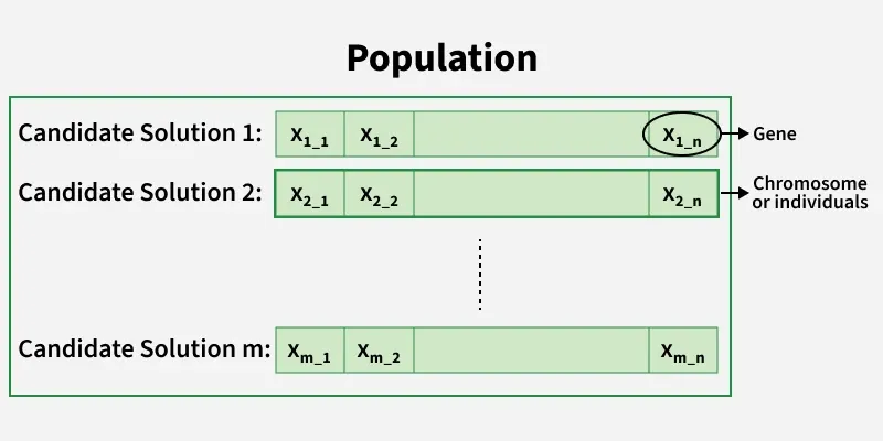
A population is a collection of candidate solutions (individuals) that exist at a particular stage (generation) of the genetic algorithm. Instead of working with a single solution, GAs simultaneously evaluate and evolve multiple solutions which helps maintain diversity and reduces the risk of getting trapped in local optima.

• Population size significantly affects convergence behavior
• Larger populations increase exploration but raise computational cost
• Smaller populations converge faster but risk premature convergence

2. Chromosome

A chromosome represents a complete candidate solution to the problem. It is a structured collection of genes that encodes all decision variables required to evaluate a solution using the fitness function.

3. Gene

A gene is the smallest unit of information in a chromosome and represents a single variable, parameteror trait of the solution. The collective behavior of all genes determines the quality of the chromosome.

4. Encoding Methods

Encoding refers to the way candidate solutions are represented inside chromosomes. Choosing an appropriate encoding is critical because it directly impacts the effectiveness of genetic operators.

a. Binary Encoding

• Uses binary strings (0 and 1)
• Simple and easy to implement
• Commonly used in theoretical GA models

b. Real-Valued Encoding

• Genes are real numbers
• Suitable for continuous optimization problems
• Faster convergence and higher precision

c. Permutation Encoding

• Chromosomes represent ordered sequences
• Used in routing, schedulingand sequencing problems
• Requires specialized crossover and mutation operators

5. Fitness Function

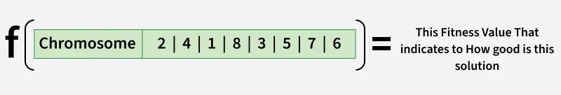
The fitness function is a mathematical formulation that evaluates how well a chromosome solves the given problem. It acts as the guiding force of the genetic algorithm by determining which individuals are more likely to reproduce.

• Higher fitness implies better solution quality
• Fitness function is problem-specific
• Can be designed for maximization or minimization

6. Termination Criteria

Termination criteria define the conditions under which the genetic algorithm stops executing. Proper termination prevents unnecessary computation while ensuring solution quality. Common termination conditions:

• Maximum number of generations reached
• Desired or threshold fitness achieved
• No improvement in fitness for several generations
• Computational time limit exceeded

7. Selection

Selection is the process of choosing chromosomes from the current population to act as parents for the next generation. The goal is to give preference to fitter individuals while still maintaining population diversity. Types of solutions include:

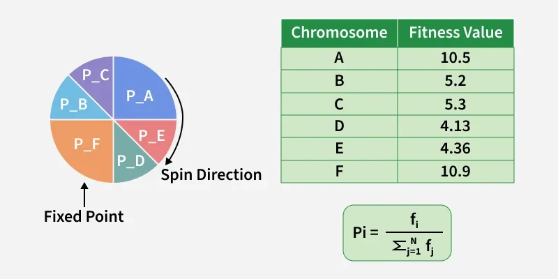
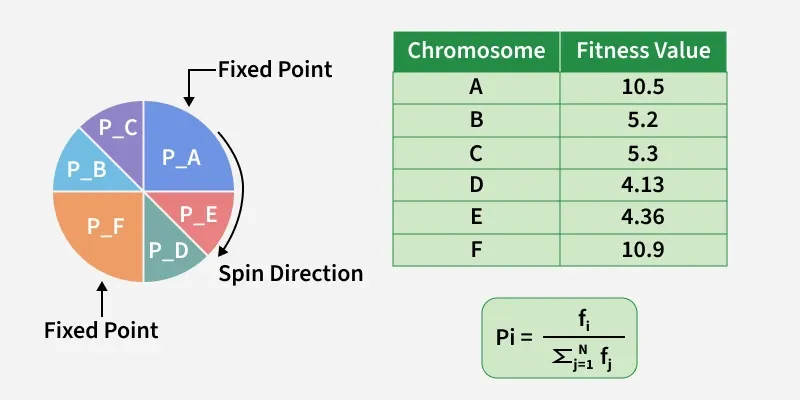
a. Roulette Wheel Selection: It is a fitness-proportionate selection technique where each individual’s probability of being selected is directly proportional to its fitness value. Individuals with higher fitness occupy larger segments of the roulette wheel, making them more likely to be chosen.

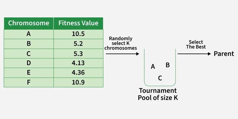
b. Tournament Selection: It randomly selects a small group of individuals from the population and chooses the fittest among them as a parent. This process is repeated until the required number of parents is selected.

c. Stochastic Universal Sampling (SUS Selection): It is an improved version of fitness-proportionate selection designed to reduce the randomness and sampling bias present in standard roulette wheel selection. Instead of using a single random pointer, SUS uses multiple equally spaced pointers to select individuals from the population.

8. CrossOver

Crossover is a genetic operator that combines genetic material from two parent chromosomes to generate new offspring. It enables the algorithm to exploit existing high-quality building blocks. Types of crossover are:

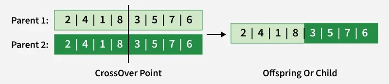
a. One Point Crossover: A random Point is chosen to be The CrossOver Point , then we fill the child with genes from both parents.

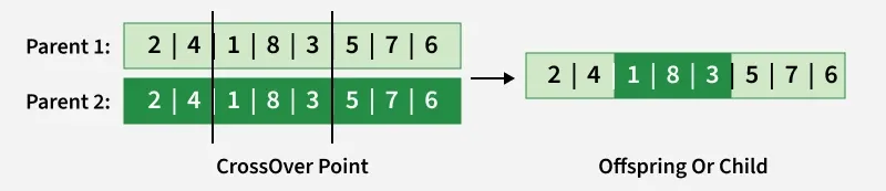
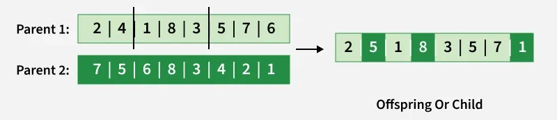
b. Multi Point Crossover: A random two Points are chosen to be The CrossOver Points , then we fill the child with genes from both parents.

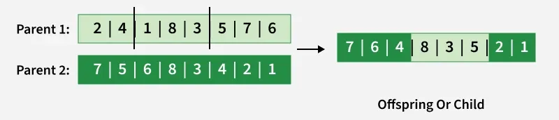
c. Davis Order Crossover (OX1): We Choose two random crossover points in the first parent and we copy that segment into the Child, then we fill the rest of genes in our child with the genes from the second Parent.

d. Uniform CrossOver: We flip a coin for each genes in our two parents to decide whether or not it’ll be included in the off-spring (Child ).

9. Mutation

Mutation introduces random changes in genes to maintain genetic diversity within the population. It helps prevent premature convergence and enables exploration of new solutions. Types of mutation are,

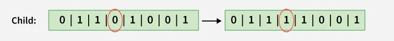
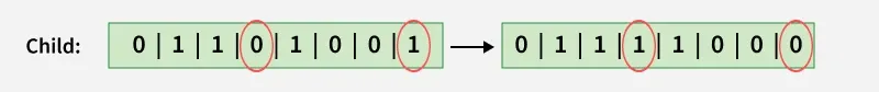
a. Bit flip Mutation: We select one or more random points (Bits) and flip them. This is used for binary encoded Genetic Algorithms.

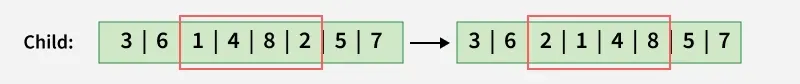
b. Swap Mutation: We Choose two Point and we switch them.

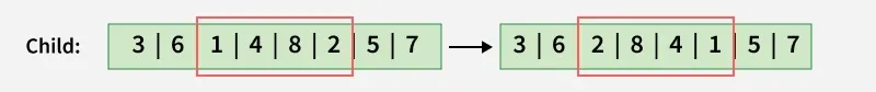
c. Scramble Mutation: We choose a random segment in The Current Chromosome and we interchange the values.

d. Inversion Mutation: We choose a random segment in The Current Chromosome and we reverse The Order of the values.

Working of Genetic Algorithms

Let's understand the working of Genetic algorithms:

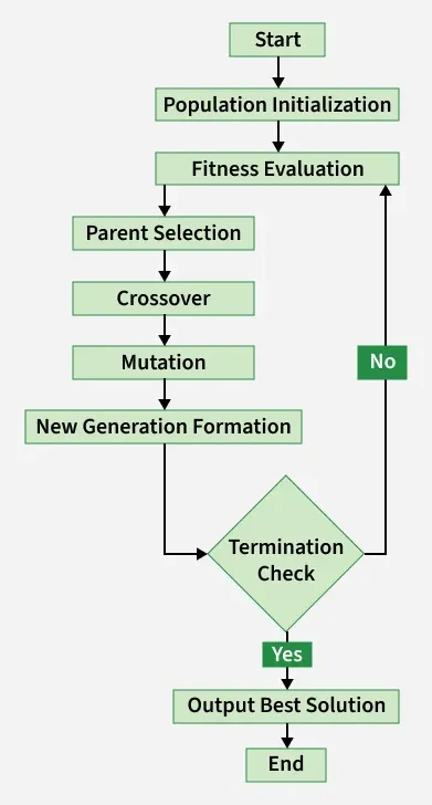
• Population Initialization: Generate an initial population of chromosomes randomly within the problem constraints.
• Fitness Evaluation: Evaluate each chromosome using the fitness function to measure solution quality.
• Parent Selection: Select parent chromosomes based on fitness using methods such as Roulette, Tournamentor SUS selection.
• Crossover: Combine genetic material from selected parents to produce offspring.
• Mutation: Apply random changes to offspring genes to maintain diversity.
• New Generation Formation: Replace the old population with newly generated offspring.
• Termination Check: Stop the algorithm if termination criteria are satisfied.
• Output Solution: Return the best chromosome obtained during evolution.

Implementation

Let's see the implementation:

Step 1: Import Libraries and Define Fitness Function

Here:

• NumPy is used for numerical computation
• Matplotlib for visualization.
• Fitness function is multimodal
• Demonstrates GA’s ability to avoid local optima

import numpy as np
import matplotlib.pyplot as plt

def fitness_function(x):
    return x * np.sin(10 * np.pi * x) + 1

Step 2: Parameter definition and population initialization

• Population size controls diversity
• Mutation and crossover probabilities regulate exploration
• Random seed ensures reproducibility

POP_SIZE = 40
GENERATIONS = 100
X_MIN, X_MAX = -1.0, 2.0
CROSSOVER_PROB = 0.9
MUTATION_PROB = 0.2
MUTATION_STD = 0.1

np.random.seed(42)
population = np.random.uniform(X_MIN, X_MAX, POP_SIZE)

Step 3: Genetic operators

• Tournament selection improves robustness
• Arithmetic crossover blends real values
• Mutation maintains diversity

def tournament_selection(pop, fitness, k=3):
    selected = []
    for _ in range(len(pop)):
        idx = np.random.choice(len(pop), k, replace=False)
        selected.append(pop[idx[np.argmax(fitness[idx])]])
    return np.array(selected)

def arithmetic_crossover(p1, p2):
    alpha = np.random.rand()
    return alpha * p1 + (1 - alpha) * p2, alpha * p2 + (1 - alpha) * p1

def mutate(x):
    if np.random.rand() < MUTATION_PROB:
        x += np.random.normal(0, MUTATION_STD)
    return np.clip(x, X_MIN, X_MAX)

Step 4: Evolution loop

• Tracks convergence behavior
• Applies full GA cycle
• Replaces old population

best_history = []
mean_history = []
for _ in range(GENERATIONS):
    fitness = fitness_function(population)
    best_history.append(np.max(fitness))
    mean_history.append(np.mean(fitness))
    parents = tournament_selection(population, fitness)
    offspring = []
    np.random.shuffle(parents)
    for i in range(0, POP_SIZE, 2):
        if np.random.rand() < CROSSOVER_PROB:
            c1, c2 = arithmetic_crossover(parents[i], parents[i + 1])
        else:
            c1, c2 = parents[i], parents[i + 1]
        offspring.extend([mutate(c1), mutate(c2)])
    population = np.array(offspring)

Step 5: Visualization

• Fitness curve shows convergence
• Scatter plot shows population distribution

x = np.linspace(X_MIN, X_MAX, 500)

plt.figure()
plt.plot(best_history, label="Best Fitness")
plt.plot(mean_history, label="Mean Fitness")
plt.legend()
plt.show()

plt.figure()
plt.plot(x, fitness_function(x))
plt.scatter(population, fitness_function(population))
plt.show()

Output:

• GA Fitness over Generations: This graph shows how fitness improves over generations. The best fitness line tracks the top solution while the mean fitness line shows the population average. Fitness rises quickly at first and then stabilizes, indicating the GA is converging.
• Final Population on Objective Function: This graph shows the final solutions on the objective function. Blue dots are the population and the highlighted point is the best individual. Most solutions cluster near high-fitness regions, showing the GA successfully found a near-optimal solution.

Applications

• Function Optimization: Used to find optimal solutions for complex, non-linear mathematical functions.
• Scheduling Problems: Applied in job scheduling, timetablingand resource allocation tasks.
• Traveling Salesman Problem (TSP): Helps determine the shortest possible route covering all cities.
• Feature Selection: Selects important features to improve machine learning model performance.
• Neural Network Optimization: Optimizes neural network weights, architectureand hyperparameters.