Normal Distribution in NumPy

The Normal (Gaussian) Distribution is a commonly used probability distribution that models natural data such as test scores, heights, sensor readings and measurement variations.

In NumPy, we generate values from a Normal Distribution using the numpy.random.normal() method, which makes it simple to create realistic, statistically consistent data for analysis and simulations.

Example: This example generates one random number from a standard normal distribution where mean = 0 and standard deviation = 1.

import numpy as np
x = np.random.normal()
print(x)

-0.972649003393483

Explanation: np.random.normal() generates one random value using default parameters loc=0 and scale=1.

Syntax

numpy.random.normal(loc=0.0, scale=1.0, size=None)

Parameters:

• loc: Mean (center) of the distribution.
• scale: Standard deviation (spread).
• size: Shape of the output (single value, list, matrix, etc.).

Examples

Example 1: This example returns one normally distributed value using default mean and standard deviation.

import numpy as np
x = np.random.normal()
print(x)

0.25448403920265805

Explanation: np.random.normal() generates one random value using default mean 0 and std 1.

Example 2: This example creates a 1-D array of five random numbers drawn from a normal distribution.

import numpy as np
arr = np.random.normal(size=5)
print(arr)

[ 1.15952571 -0.08602516 -1.52141403 -1.24343932  0.43504395]

Explanation: size=5 produces an array containing 5 normally distributed values.

Example 3: This example generates a 2×3 matrix with mean = 10 and standard deviation = 2, useful for simulations.

import numpy as np
m = np.random.normal(loc=10, scale=2, size=(2, 3))
print(m)

[[ 9.65291001  8.83304941 13.11063692]
 [ 6.23383207  9.80784053 11.20479514]]

Explanation:

• loc=10 shifts the distribution’s center to 10.
• scale=2 spreads values around the mean with std = 2.
• size=(2,3) produces a 2×3 matrix.

Visualizing the Normal Distribution

Visualizing the generated numbers helps in understanding their behavior. Below is an example of plotting a histogram of random numbers generated using numpy.random.normal.

import numpy as np
import matplotlib.pyplot as plt
from scipy.stats import norm

# Generate data
data = np.random.normal(loc=0, scale=1, size=1000)

# Plot histogram
plt.hist(data, bins=30, edgecolor='black', density=True)

# Plot theoretical PDF
x = np.linspace(-4, 4, 200)
pdf = norm.pdf(x, loc=0, scale=1)
plt.plot(x, pdf, label="Theoretical PDF")

plt.title("Normal Distribution")
plt.xlabel("Value")
plt.ylabel("Density")
plt.grid(True)
plt.legend()
plt.show()

Output

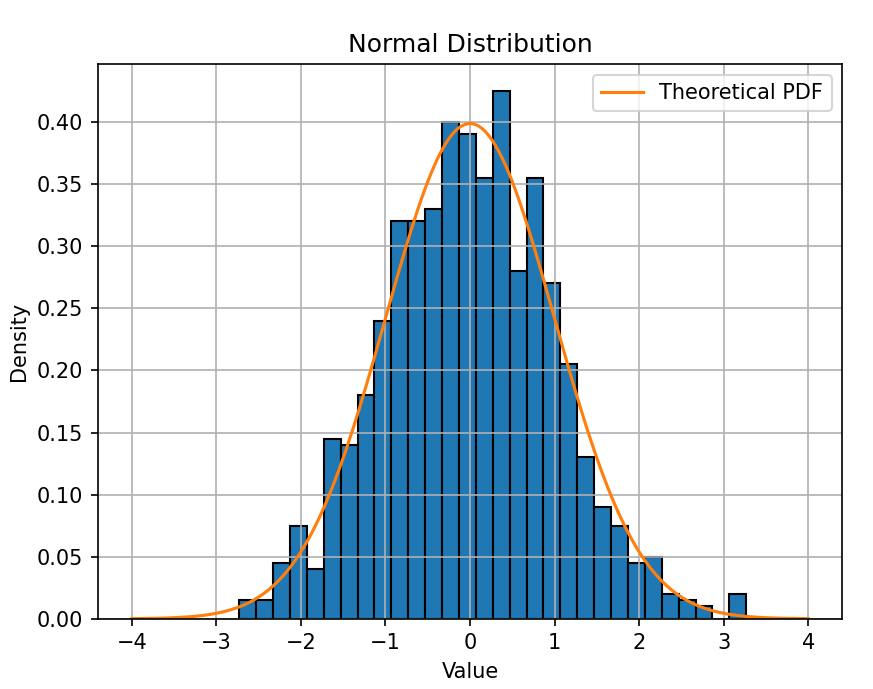
Explanation:

• np.random.normal(loc=0, scale=1, size=1000) generates 1000 values following a standard normal distribution.
• plt.hist(data, density=True) plots the frequency of values, normalized to form a density curve.
• norm.pdf(x, loc=0, scale=1) computes the theoretical bell curve for comparison.
• Plotting both together shows how closely the generated random numbers follow the actual normal distribution.