Digital morphogenesis studies how forms, shapes, and patterns emerge in nature through computational models of biological, chemical, and physical processes, with applications in architecture, fabrication, art, engineering, biomedicine and more.
This list is a compact reference of growth algorithms, lab experiments, and related math/physics/programming topics so readers can find unexpected relationships and patterns across disciplines.
Contributions are welcome! If you have improvements, links, or missing topics to add, please open an issue or PR.

Note
Related to Diffusion-limited aggregation (DLA) and Laplace equation.
Image credit: Ellak Somfai - Dielectric breakdown model in 3 dimensions.
Generalization of DLA that models how an electrical discharge propagates through an insulating (dielectric) material, producing the branching patterns known as Lichtenberg figures - the same kind of patterns seen in lightning, fulgurites in sand, and burn marks left by high-voltage discharge.
Rather than growing a cluster from randomly-walking particles like DLA, DBM solves Laplace's equation for the electric potential around the growing cluster at every step, then extends growth from whichever boundary site has the strongest local field.
A single exponent, η (eta), controls how sharply growth concentrates at high-field points: at η = 1 the model is statistically equivalent to DLA, higher values produce sparser and more needle-like branches, and η = 0 produces smooth, non-fractal growth.
Algorithm at a glance:
* indicates a potential simulation parameter
- Seed growth with an initial charged point or shape, and hold a distant boundary* at zero potential (fully "discharged").
- Solve for the potential field filling the space around the cluster - either by repeatedly relaxing a grid (each free cell settles toward the average* potential of its neighbors, over some number of iterations*) until the field stabilizes, or by approximating it with a batch of random walkers* launched from the boundary and recording where each one first touches the cluster.
- For each empty cell touching the cluster (a "candidate" site), calculate its local field strength as how much its potential has dropped relative to the cluster's fixed potential.
- Raise each candidate's field strength to the power of the growth exponent* (η), normalize the results into probabilities, and randomly pick one (weighted by those probabilities) to add to the cluster.
- Repeat, resolving the field again after each new addition.
Key terms:
- η (eta) - exponent controlling how strongly growth favors high-field regions; DLA is the η = 1 case of DBM.
- Lichtenberg figure - branching discharge pattern that DBM was originally developed to explain.
- Rigid and elastic bond models - DBM variants used to study electrical and mechanical breakdown (fracture) networks.
Articles:
- Dielectric breakdown model on Wikipedia
- Lichtenberg figure on Wikipedia
- Fractal Dimension of Dielectric Breakdown (PDF) by L. Niemeyer, L. Pietronero, and H. J. Wiesmann. The original 1984 paper introducing DBM as a generalization of DLA.
Code projects:
- Lichtenberg-Figures - DBM-based simulation of Lichtenberg figure formation, accounting for the stochastic nature of dielectric breakdown

Note
Related to Dielectric breakdown model (DBM) and Laplace equation.
Process in which particles of matter stick together (aggregate) as they chaotically move (diffuse) through a medium that provides some sort of resistive (limiting) force. As these particles clump together over time they form characteristic fractal branching structures known as Brownian trees.
Very interesting macro-structures begin to emerge at around the 1-10 million particle range in 3D, but in order to get there you'll need to be smart about your rendering pipeline and make use of optimized code in a performant language or environment (C/C++, CUDA, GLSL shaders, Houdini, etc).
Algorithm at a glance:
- Add initial point(s) or shapes to seed growth.
- Add a number of walker particles.
- In each tick of the simulation, do the following:
- Move each walker a small amount in a random direction.
- If any walker particle is colliding with a fixed/clustered particle, convert that walker particle into a fixed/clustered particle.
Key terms:
- Walker - randomly-moving particle not attached to any other particle
- Cluster - group of multiple particles stuck together
- Brownian tree - name of characteristic branching structure that emerges
Articles:
- Diffusion-limited aggregation on Wikipedia
- Diffusion-Limited Aggregation, a Kinetic Critical Phenomenon (1981) by Thomas Witten and Leonard Sander. The article that started it all! Note: visit your local library or a university library and ask a librarian if they can help you get free access!
- Diffusion-limited aggregation: A kinetic critical phenomenon? (2000) by Leonard Sander. Follow-up to the original article.
- Simulating 2D diffusion-limited aggregation (DLA) with JavaScript by Jason Webb
- DLA - Diffusion Limited Aggregation by Paul Bourke
- Diffusion-Limited Aggregation by Softology
- Pushing 3D Diffusion-Limited Aggregation even further by Softology
Code projects:
- dlaf (C++ w/ Boost) by Michael Fogleman
Introduces a novel, super-efficient method of collision detection, described here. - 2D diffusion-limited aggregation (DLA) experiments in JavaScript (Github repo) by Jason Webb
- simutils-0001: Diffusion limited aggregation by Karsten Schmidt (toxiclibs)
- Simulate: Diffusion-Limited Aggregation from FORM+CODE book examples
- Dendron Processing sketch by Golan Levin
Creative projects:
- Aggregation series by Andy Lomas
Notable software:
- Visions of Chaos
- glChAoS.P by Michele Morrone (BrutPitt)
Videos:
- Coding Challenge #34: Diffusion-Limited Aggregation by Daniel Shiffman (Github repo)
- Coding Challenge #127: Brownian Tree Snowflake by Daniel Shiffman (Github repo)
- VEX in Houdini: Diffusion Limited Aggregation (Plus Rendering In Mantra & Redshift) by Entagma

Process that acts on continuous chains of nodes connected by lines using simple rules (attraction, repulsion, alignment; not unlike boids) in order to produce undulating, buckling forms that mimic or simulate meandering rivers, rippled surface textures of plants/seeds/fruits, space-filling behaviors of worms, snakes, intestines, and much more.
Algorithm at a glance:
2D:
- Begin with a set of nodes connected in a chain-like fashion to form a path (or multiple paths). Each node should have a maximum of two neighbors (one preceding, one following).
- In each tick of the simulation, for each node:
- Move node towards it's connected neighbor nodes (attraction).
- If node gets too close to any nearby nodes (connected or not), move it away from them (repulsion).
- Move node towards the midpoint of an imaginary line between it's preceding and following nodes (alignment). It wants to rest equidistance between them with as little deflection as possible.
- In each tick of the simulation, evaluate the distances between each pair of connected nodes. If too great, insert a new node between them (adaptive subdivision).
- At some interval, insert new nodes in the chain to over-constrain the system and induce growth. The bends and undulations that emerge are a result of the system trying to equalize the forces using the rules defined in step 2.
Articles and discussions:
- Exploring 2D differential growth with JavaScript by Jason Webb
- Differential line by Anders Hoff (inconvergent)
- Sheparding Random Growth by Anders Hoff (inconvergent)
- Differential Mesh Growth discussion thread on od|force forums
- Organic Labrynths and Mazes (PDF) paper by Hans Pederson and Karen Singh
Code projects:
- 2D differential growth experiments by Jason Webb (Github repo)
- Differential line growth with Processing by Alberto Giachino
- Real-time differential growth in JavaScript by Adrian Toncean
- Differential Line Growth by Maritz Schwind of Entagma
- Differential Growth by Lionel Radisson
Creative projects:
- Floraform - an exploration of differential growth by Nervous System
- Floraform Chandelier at World Expo 2017 in Astana, Kazakhstan by Nervous System
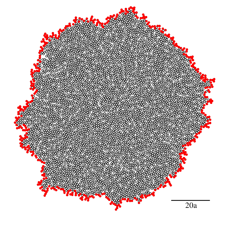
Image credit: Silvio Costa Ferraria et al - Figure 1 from Pitfalls on the determination of the universality class of radial clusters
Created by Murray Eden in 1961 (paper (PDF)), this is a type of surface fractal growth process where material randomly accumulates on the boundary of clusters. Sort of like DLA but without all the empty space between branches. Thought to be a good way to model certain kinds of bacterial and lichen growth.
Algorithm at a glance:
* indicates a potential simulation parameter
- Seed growth with a single occupied cell (or shape).
- Track the list of all empty cells touching the cluster - its "perimeter."
- Pick one perimeter cell to fill in - either uniformly at random*, or weighted by how many cluster cells it touches* - and add it to the cluster.
- Update the perimeter list: remove the cell just filled, and add any new empty cells it exposed.
- Repeat.
Key terms:
- Perimeter / boundary sites - the empty cells adjacent to the cluster; the pool of candidates for the next growth step.
- Growth-site weighting - how a perimeter cell is chosen each step; picking uniformly among all perimeter cells produces a different texture than weighting by how many cluster neighbors a cell has.
- Kardar–Parisi–Zhang (KPZ) universality class - broad category of surface-growth models that share the same statistical scaling behavior; the Eden model is a classic example used to study it.
Articles:
- Eden growth model on Wikipedia
- A Two Dimensional Growth Process by Murray Eden (original 1961 paper)
Code projects:
- Eden_cluster_growthtests - Python implementation with a repulsion factor to model canopy shyness in trees

Note
Related to Primordial Particle System and agent-based modelling.
Image credit: detail of the example results from Particle Life Simulation by Hunar Ahmad
Family of particle systems in which every particle belongs to one of several types (usually drawn as colors), and every ordered pair of types is assigned its own attraction or repulsion strength. Those strengths are held in a small matrix that can be filled randomly and then tuned by hand, which makes the system extremely easy to explore - each new matrix is effectively a new set of "physics" to play with.
Crucially, the matrix does not have to be symmetric: green can be attracted to red while red is repelled by green. That asymmetry is what lifts the results beyond simple clumping, producing cell-like clusters with membranes, wandering "creatures" that chase and flee each other, orbiting pairs, snaking chains, and blobs that pinch off copies of themselves - all within one parameter space.
Originally explored by Jeffrey Ventrella as Clusters and later popularized under the name "Particle Life" by CodeParade in 2018, this is one of the most approachable emergent systems to implement, since the core is just a nested loop over pairs of particles.
Not to be confused with the Primordial Particle System, which uses a single kind of particle steering by neighbor counts - here the effects depend entirely on multiple types treating each other differently.
Algorithm at a glance:
* indicates a potential simulation parameter
- Randomly place a number* of particles, assigning each one of
k* types (colors). - Build a
k × kmatrix* of attraction values (commonly in the range-1to1), one for each ordered pair of types, where negative values mean repulsion. Random matrices are a good starting point, and the matrix need not be symmetric. - In each tick of the simulation, for each particle:
- Find nearby particles within a maximum interaction radius*.
- For each neighbor, compute a force: strong repulsion when closer than some minimum distance* (so particles cannot collapse into a single point), and beyond that, an attraction or repulsion scaled by the matrix value for the pair of types involved. The exact shape of the falloff curve varies between implementations and has a big impact on the results.
- Add the summed forces to the particle's velocity, apply friction/damping*, then move it.
- Wrap or bounce particles at the edges of the world*.
Key terms:
- Types (or families/colors) - the classes of particle whose interactions the matrix describes
- Attraction matrix -
k × ktable of per-pair attraction and repulsion strengths - Minimum distance - radius inside which particles always repel each other
- Maximum radius - distance beyond which particles ignore each other, usually enforced with a spatial index
- Friction - velocity damping, without which the system heats up and flies apart
Articles:
- Clusters by Jeffrey Ventrella - the original system, along with an introduction to the ideas behind it
- Clusters and Particle Life by Softology - traces the lineage from Clusters to Particle Life and walks through the parameters
Videos:
- Particle Life - A Game of Life Made of Particles by CodeParade
- Clusters: An Asymmetrical Particle System with Emergent Patterns by Jeffrey Ventrella
- Particle Life Simulation by Hunar Ahmad - code walkthrough of an implementation that fits on a page
Projects:
- Particle Life by Veronica Lin, based on particle-life-sim.
- Particle Life Simulation (C++, JavaScript, and Python) by Hunar Ahmad - includes browser demos in 2D and 3D
- Particle Life (Java) by Tom Mohr - desktop app using parallel processing and spatial partitioning to handle large particle counts (Github repo), built on a reusable framework
- Particle-Life (C++) by CodeParade - the implementation from the video above

Image credit: Sage Jenson (@mxsage)
Technique for modelling the observed behaviors of the slime mold physarum polycephalum using agent-based modelling. Originally described in 2010 paper by Jeff Jones, and more recently popularized by artist Sage Jensen (@mxsage), this algorithm produces highly dynamic and organic-looking webs that can seem very life-like and biological in nature.
Algorithm at a glance:
* indicates a potential simulation parameter
- Consider the simulation space as a grid, with each cell storing a number representing the combined strength of pheromones left by the agents who have passed through it.
- Pheromones in each cell diffuse at some rate* to neighboring cells as they decay (at some rate*) in each step of the simulation.
- Add a set of points, each representing an autonomous agent.
- Each agent leaves a trail of decaying pheromones behind by adding a number* to the cells it passes through.
- Each agent senses the total phermone strength of cells in front of it defined by a distance* and a field of view angle*.
- An agent will gradually adjust its direction* to steer towards the cell(s) with the most pheromones.
- Render the trails (not the agents) by mapping the pheromone strength number in each cell to a range or gradient of colors.
Articles:
- Characteristics of Pattern Formation and Evolution in Approximations of Physarum Transport Networks (PDF) by Jeff Jones - original paper
- Physarum Simulations by Softology
- Physarum polycephalum on Wikipedia
- Understanding the Physarum Simulation by Deniz Bicer (breakdown thread)
Code projects:
- Simulating slime mold with WebGL by Ken Voskuil
- physarum (JavaScript with ThreeJS) by Nicolas Barradeau
- Physarum (Unity) by Deniz Bicer
- Physarealm (Rhino + Grasshopper) by Ma Yidong
- Physarum (C++, with 2D and 3D implementations) by Jan Ivanecky
Creative projects:
- physarum by Sage Jenson (mxsage)
- Slime mold by Georgios Cherouvim

Note
Related to Particle Life and agent-based modelling.
Image credit: detail of Figure 3G from Schmickl, Stefanec & Crailsheim (2016)
Described in 2016 by Thomas Schmickl, Martin Stefanec and Karl Crailsheim of the Artificial Life Lab in Graz, Austria, a Primordial Particle System (PPS) is a minimal agent-based model in which self-propelled particles move through continuous space while steering based only on how many neighbors they can see to their left and right - a motion law even simpler than boids, with no cohesion, separation or alignment rules. It is a separate system from Particle Life, where all of the behavior comes instead from multiple particle types with per-pair attraction rules.
Despite containing no notion of cells, membranes or reproduction, the system spontaneously produces cell-like structures with a dense interior surrounded by a ring-like membrane, and those structures go through a full life cycle: they feed on the surrounding "nutrient" field of free particles, grow, divide into daughter cells and spores, and die when starved. Left running, the population of cells levels off along a sigmoidal curve much like bacteria growing in a petri dish, making this one of the most striking demonstrations of how self-structuring, self-reproducing and self-sustaining behaviors can emerge from a single line of math.
Motion law:
Where
Algorithm at a glance:
* indicates a potential simulation parameter
- Randomly distribute particles across the habitat with random headings, at a density* of around 0.08 particles per square unit (the paper uses a 250x250 unit space that wraps around at the edges).
- In each time step, visit every particle once, in random order, and for each one:
- Count its neighbors within radius
$r$ *, splitting them into those on its left ($L$ ) and those on its right ($R$ ). - Turn it by
$\Delta\phi$ using the motion law above, with a fixed angle$\alpha$ * and a crowding-proportional angle$\beta$ *. - Move it forward by a constant velocity
$v$ *.
- Count its neighbors within radius
- Update particles asynchronously - each particle senses and moves within the same loop, so it sees the already-updated positions of the particles visited before it in that time step. Updating everything simultaneously instead will not produce the same results.
- Optionally color-code particles by local neighborhood size to make the structures legible (see below).
Reference parameter set:
Color coding (as used in the paper):
- Green (
$N \leq 13$ ) - free-floating "nutrient" particles - Brown (
$13 \leq N \leq 15$ ) - premature spores - Magenta (more than 15 neighbors within a much smaller radius of 1.3) - mature spores
- Blue (
$15 < N \leq 35$ ) - the bulk of cell structures, including their membranes - Yellow (
$N > 35$ ) - the densest interiors of cells
Articles:
- How a life-like system emerges from a simple particle motion law by Thomas Schmickl, Martin Stefanec & Karl Crailsheim - original 2016 paper in Scientific Reports (open access, with pseudo-code in Figure 1).
- Primordial Particle Systems research track page from the Artificial Life Laboratory in Graz, Austria.
- A Primordial Particle System in three dimensions by Thomas Schmickl & Martin Stefanec - extends the model into 3D, with pseudo-code and notes on what has to change.
- Complexity by Thomas Schmickl - short plain-language introduction from one of the authors.
Videos:
- How life emerges from a simple particle motion law: Introducing the Primordial Particle System by the Artificial Life Lab Graz
Projects:
- Primordial Particle System (JavaScript, single-page HTML canvas) by nagualdesign (Github repo)
- emergence (C++ with OpenGL and OpenCL) by blobject - PPS visualiser and processor with live parameter controls
- pps (Go, renders in the browser) by fzipp
- PPS (Processing) by Adam Brown
- pml_system (C) by Timo Lassmann
- PrimordialParticleSystems_Public by Thomas Schmickl - implementations shared by one of the original authors

Note
Related to convolution kernel and Laplace equation.
Grid-based process that generates complex and dynamic patterns based the interactions of two chemicals as they diffuse through a medium and react with one another. At every location on the grid these chemicals (usually referred to as A and B) have a chance of causing a reaction that converts chemicals of one type to another based on their relative concentrations at that location.
Throughout the simulation chemical A is added at a particular feed rate (f) and chemical B is removed at a particular kill rate (k) - adjusting these rates can result in wildly different emergent patterns.
Equation (via Karl Sims):

Key terms:
- Feed rate - rate at which chemical
Ais added to system - Kill rate - rate at which chemical
Bis removed from the system - Diffusion rate - rate at which each chemical spreads, which acts as a kind of scaler to a 3x3 Laplacian transform
- Reaction chance - probability that one
Awill be converted to aBwhen in the presence of twoBs. - Gray-Scott model
- Pearson's classification
- Turing patterns
Articles:
- Reaction-diffusion system on Wikipedia
- Reaction-Diffusion Tutorial by Karl Sims
- Reaction-Diffusion by the Gray-Scott Model: Pearson's Parametrization by Robert Munafo (mrob)
- Reaction Diffusion: The Gray-Scott Algorithm by Algosome
- The Chemical Basis of Morphogenesis (PDF) paper by Alan Turing (1952)
Notable tools:
Code projects:
- Gray–Scott Reaction Diffusion (JavaScript + WebGL) by Mike Bostock
- Gray-Scott - JavaScript experiments by @pmneila
- simutils-0001: Gray-Scott reaction diffusion by toxiclibs
- ofxReactionDiffusion add-on for openFrameworks by Yuma Matsune
- ofxRD add-on for openFrameworks by aanri
- Reaction Diffusion (JavaScript + WebGL) by Red Blob Games
- Reaction Diffusion by Ken Voskuil (look in the DOM)
- Reaction-Diffusion Playground (JavaScript, ThreeJS/WebGL, shaders) by Jason Webb
- Reaction-Diffusion Simulation in Three.js (JavaScript + ThreeJS) by Jonathan Cole
- Reaction diffusion with C++ and SFML by Deedone
- Reaction-Diffusion simulation with C++, SFML, & Cuda by Luka Mattfield (@Solidsilver)
- ReaDDy (C++ with Python bindings)
- RDSystem (Unity) by Keijiro Takahashi
- Multiscale Turing Patterns (JavaScript, GLSL, regl) by Ricky Reusser
- Read his write-up and try the live version here.
- Available on Observable too.
Creative projects:
- Jonathan McCabe's multi-scale Turing pattern series. See Diatomaceous, Bone Music [2] [3], Multi-Scale Turing Patterns and others
- See his paper Cyclic Symmetric Multi-Scale Turing Patterns (PDF), and this post from Softology explaining it.
- 3D Printed Reaction Diffusion Patterns Instructable by Reza Ali
- Processing: Reaction Diffusion Halftone patterns by Ignazio Lucenti
- Coral Cup by Nervous System
- Reaction Lamps by Nervous System
- Reaction Table and reaction shelf by Nervous System
- Reaction-Diffusion Media Wall by Karl Sims
- DIFFUSION by Kouhei Nakama
- Reaction Diffusion using point clouds by David Grzesik. See his write-up here (PDF)
- Grey Scott’s Reaction Diffusion - Houdini VEX by Ali Seiffouri
- Healing series by Brian Knep
- Silhouect by Justin Gitlin (@cacheflowe)
- Reaction diffusion by Artur Żarejko
Videos:
- Fun with Reaction-Diffusion in Houdini by Dan Willis at SIGGRAPH Asia 2019.
- Reaction Diffusion video series for Houdini by Entagma:
- Coding Challenge #13: Reaction Diffusion Algorithm in p5.js by Daniel Shiffman (Github repo with both p5.js and Processing source code)
- Reaction Diffusion: A Visual Explanation by Arsiliath

Process for iteratively growing networks of branching lines based on the distribution of growth hormone sources (called "auxin" sources) to which the lines are attracted. Originally described by Adam Runions and collaborators at the Algorithmic Botany group at the University of Calgary, this system can be used to simulate the growth of leaf venation patterns and tree-like structures, as well as many other vein-like systems like Gorgonian sea fans, circulatory systems, root systems, and more.
The original algorithm describes methods for generating both "open" (as seen in the example GIF) and "closed" venation networks, referring to whether or not secondary or tertiary veins connect together to form loops (or anastomoses).
Algorithm at a glance:
For both the open and closed variants of this algorithm, begin by placing a set of points on the canvas representing sources of either the auxin growth hormone (as in leaves) or ambient nutrients (as in trees).
Open venation:
- Associate each auxin source with the single closest vein segment within a pre-defined attraction distance.
- For each vein segment that is associated with at least one auxin source, calculate the average direction towards them as a normalized vector and generate a new vein segment that extends in that direction at a pre-defined segment length (by scaling the normalized direction vector by that length).
- Remove any auxin sources that have vein segments within a pre-defined kill distance around it.
Closed venation:
- Associate each auxin source with all of the vein segments that are both within a pre-defined attraction distance and within the source's relative neighborhood.
- For each vein segment that is associated with at least one auxin source, calculate the average direction towards them as a normalized vector and generate a new vein segment that extends in that direction at a pre-defined segment length (by scaling the normalized direction vector by that length).
- Remove any auxin sources that have been reached by all of their associated vein segments.
Auxin flux canalization:
- Give each vein segment a uniform default thickness to start with.
- Beginning at each terminal vein segment (that is, segments with no child segments), traverse "upwards" through each parent vein segment, adding their child vein segment thickness to their own until you reach a root vein segment (a segment with no parent segment).
Key terms:
- Auxin source = a discrete location towards which vein segments are attracted. In biology, auxin is a hormone found in plants that promotes growth.
- Auxin flux canalization = process by which veins become thicker as they grow longer. The longer a vein gets, the more auxin flows through it ("flux"), causing veins to progressively thicken from their tips to their roots. "Canalization" references the process by which "canals" of water form.
- Relative neighborhood = point P is a relative neighbor of a point Q if there is no other point R closer to P and Q than they are to each other.
Articles and papers:
- Modeling and visualization of leaf venation patterns (PDF) original 2005 paper by Adam Runions, Martin Fuhrer, Brendan Lane, Pavol Federl, Anne−Gaëlle Rolland−Lagan, and Przemyslaw Prusinkiewicz
- Modeling Trees with a Space Colonization Algorithm (PDF) 2007 paper by Adam Runions, Brendan Lane, and Przemyslaw Prusinkiewicz
- Modeling organic branching structures with the space colonization algorithm and JavaScript by Jason Webb
- Procedurally Generated Trees with Space Colonization Algorithm in XNA C# by Jon Gallant
- Part 26: Trees by Michael Goodfellow
- Art-directing procedural vegetation in Houdini using a space colonization algorithm (PDF) by Marta Feriani
Creative projects:
- Hyphae and Xylem series by Nervous System
- Also see their Xylem Experiments and Improvements write-up
- Bromeliad and Calyx lamps by Nervous System
Code projects:
- ofxSpaceColoinzation add-on for openFrameworks
- space-colonization (JavaScript) by Nick Nikolov
- Dendrite (Unity) by mattatz
- Grower (Maya plugin) by Jose Esteve
- Venation (Processing) by Niel McLaren
- hyphae (Julia) by Jamie Blondin
- hyphae and hyphae_ani by Anders Hoff (inconvergent)
- 2d-space-colonizations-experiments (JavaScript) by Jason Webb
Videos:
- Coding Challenge #17: Fractal Trees - Space Colonization by Daniel Shiffman (Github repo with source code for p5.js and Processing)

String rewriting system invented by biologist Aristid Lindenmayer in 1968 to model the growth processes of plant development and other organisms. L-systems use simple grammatical rules to iteratively expand a string of symbols, which can then be interpreted geometrically (e.g., using turtle graphics) to produce complex branching structures. Despite their simplicity, L-systems can generate remarkably naturalistic plant forms, fractals, and branching patterns.
The key insight is that local production rules (each symbol rewrites to a sequence of symbols) applied recursively across iterations can generate globally complex structures without explicitly encoding the final form. This makes L-systems particularly powerful for modeling hierarchical biological growth.
Algorithm at a glance:
* indicates a potential simulation parameter
- Define an axiom* - the initial string (often just "F" or a single symbol).
- Define production rules* - for example, "F → FF" (each forward step becomes two forward steps).
- Define a number of iterations*.
- For each iteration, replace every symbol in the string according to its production rule, simultaneously.
- Interpret the final string geometrically:
- Common symbols:
F(move forward and draw),f(move forward without drawing),+(turn left),-(turn right),[(push position/heading to stack),](pop position/heading from stack)
- Common symbols:
- Render the resulting path or tree structure.
Example:
| Description | Rendered Result |
|---|---|
Axiom: FRule: F → F[+F]F[-F]FAfter iteration 1: F[+F]F[-F]FAfter iteration 2: F[+F]F[-F]F[+F[+F]F[-F]F]F[+F]F[-F]F[-F[+F]F[-F]F]F[+F]F[-F]FWhen rendered with angle=25°, this produces a branching plant-like structure. |
 |
Key terms:
- Axiom - the starting string
- Production rules - symbol-to-string mappings applied each iteration
- Turtle graphics - geometric interpretation of the L-system string using position, heading, and a drawing pen
- Stochastic L-systems - rules chosen probabilistically rather than deterministically, creating variation
- Parametric L-systems - rules can use parameters and conditions for more sophisticated generation
- Context-sensitive L-systems - rules depend on neighboring symbols, allowing more complex interactions
Articles:
- L-system on Wikipedia
- Chapter 1: Plant Models from Algorithmic Botany book - foundational reference
Videos:
- Coding Challenge #16: Recursive Trees - Fractal Trees by Daniel Shiffman (Github repo with p5.js and Processing code)
- L-System Creature Evolution by Lenia
- 8.5: L-Systems from Daniel Shiffman's Nature of Code series
Notable tools and libraries:
- Blender
- Sapling Tree Gen - add-on for procedural L-system-based tree generation
- Houdini
- TouchDesigner
- Unity
- SpeedTree - commercial procedural tree generator with L-system-based generation
- Unreal Engine
- SpeedTree integration - native support for SpeedTree models

Note
Related to reaction-diffusion.
Physical process by which a homogeneous mixture (a molten alloy, polymer blend, glass, etc.) spontaneously separates into two distinct phases when rapidly cooled ("quenched") into an unstable region of its phase diagram. Unlike typical nucleation-based phase separation, no discrete starting sites or thermodynamic barrier are needed - tiny composition fluctuations grow everywhere in the material simultaneously.
The result is a characteristic pattern of intertwined, worm-like regions that grow and merge ("coarsen") over time while roughly maintaining the same overall proportions of each phase - visually similar to some reaction-diffusion patterns, though it arises from a different underlying process (phase-separation thermodynamics rather than a chemical feed/kill reaction). It's commonly modeled with the Cahn-Hilliard equation, a PDE describing how the concentration of the two phases diffuses and separates over time.
Algorithm at a glance:
* indicates a potential simulation parameter
- Fill a grid with random noise* representing the initial, unstable composition of the mixture.
- At each step, for every cell, calculate how its concentration should change based on two competing effects: diffusion (smoothing out differences with its neighbors) and phase separation (pushing its value away from the mixed middle and toward one pure phase or the other).
- Update every cell by combining these two effects, scaled by a diffusion rate* and a phase-separation strength*.
- Repeat, letting separated regions grow and merge (coarsen) over time.
Key terms:
- Cahn-Hilliard equation - the PDE most commonly used to model spinodal decomposition.
- Quench - rapid cooling of a mixture into an unstable region of its phase diagram, triggering decomposition.
- Coarsening - the slow, ongoing growth and merging of separated regions over time.
- Nucleation - the barrier-driven alternative to spinodal decomposition, where phase separation starts at discrete sites rather than everywhere at once.
Articles:
- Spinodal decomposition on Wikipedia
- Cahn-Hilliard equation on Wikipedia
- Spinodal decomposition generative art post on r/generative - the post that inspired this topic's request
Code projects:
- Spinodal-Decomposition (MATLAB) by Nicholas Balbi - simulates and renders the Cahn-Hilliard equation

Note
Related to polyhedra and Platonic solids.
Set of 13 semi-regular convex polyhedra composed of regular polygons meeting in identical vertices, excluding the 5 Platonic solids (which are composed of only one type of polygon) and excluding the prisms and antiprisms.
Each shape can be constructed by starting with one of the Platonic solids and truncating it's corners or edges in various ways.
List of Archimedean solids:
| Name | Faces | Edges | Vertices | Image |
|---|---|---|---|---|
| Truncated tetrahedron | 4 triangles 4 hexagons |
18 | 12 |  |
| Cuboctahedron | 8 triangles 6 squares |
24 | 12 |  |
| Truncated cube | 8 triangles 6 octagons |
36 | 24 |  |
| Truncated octahedron | 6 squares 8 hexagons |
36 | 24 |  |
| Rhombicuboctahedron | 8 triangles 18 squares |
48 | 24 |  |
| Truncated cuboctahedron | 12 squres 8 hexagons 6 octagons |
72 | 48 |  |
| Snub cube | 32 triangles 6 squares |
60 | 24 |  |
| Icosidodecahedron | 20 triangles 12 pentagons |
60 | 30 |  |
| Truncated dodecahedron | 20 triangles 12 decagons |
90 | 60 |  |
| Truncated icosahedron | 12 pentagons 20 hexagons |
90 | 60 |  |
| Rhombicosidodecahedron | 20 triangles 30 squares 12 pentagons |
120 | 60 |  |
| Truncated icosidodecahedron | 30 squares 20 hexagons 12 decagons |
180 | 120 |  |
| Snub dodecahedron | 80 triangles 12 pentagons |
150 | 60 |  |
Articles:
- Archimedean solid on Wikipedia
- Archimedean Solid on Wolfram MathWorld
- Archimedean Polyhedra by George Hart
Videos:
- Platonic and Archimedean solids by Henry Segerman
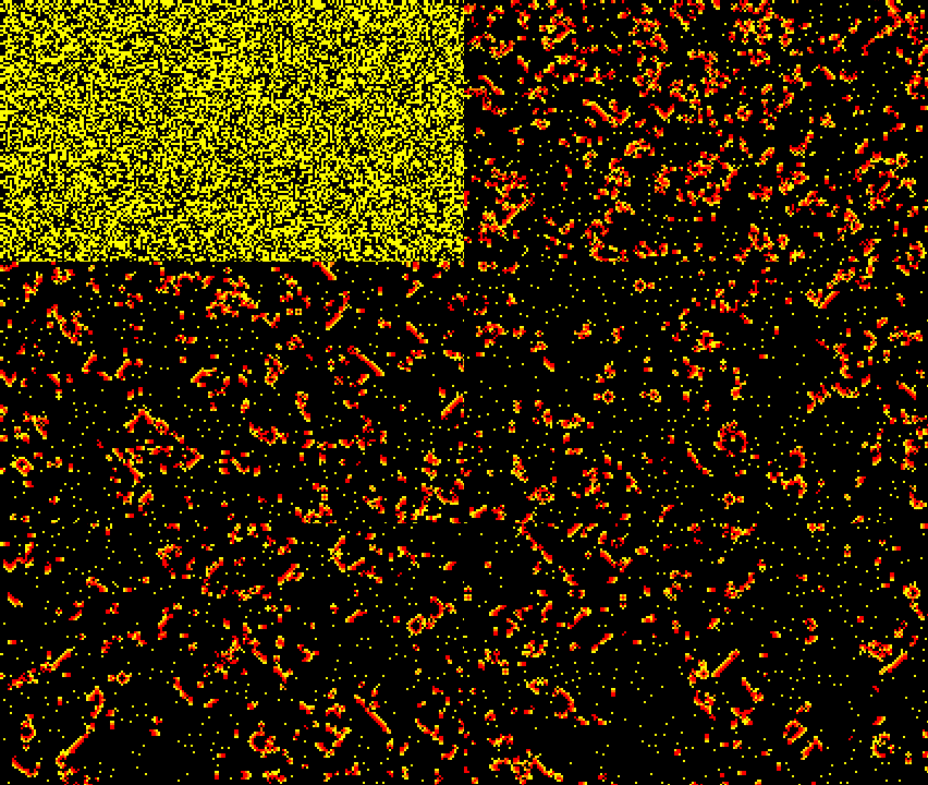
Note
Related to convolution kernel.
A regular grid of cells with states that are updated each iteration in according to rules. Developed by Stanislaw Ulam and John von Neumann at the Los Alamos National Laboratory in the 1940s, this system has been used to model physical, biological, and social phenomena with remarkable variety and accuracy.
Key terms:
- Cell - a discrete location on the grid
- State - the "value" of a cell. Many CAs just have two states (on/off), but others use many.
- Neighborhood - set of cells surrounding a given cell. Most common types are Von Neumann and Moore, though others exist.
- Rule(s) - mathematical functions or if/else statement(s) that define what the next state of a cell should be based on various criteria like the states of that cell's neighbors. Sometimes called transition rules.
- Generation - result of one iteration of the system.
Types:
- Asynchronous - automaton in which each cell is updated independantly of the others over time. Multiple update schemes have been proposed by various researchers.
- Block - automaton in which the grid of cells is divided into non-overlapping blocks, with rules being applied to entire blocks rather than individual cells. Also known as a partitioning cellular automaton.
- Continuous - automaton in which each cell has a real number value instead of an integer state.
- Continuous spatial - automaton in which the cell locations are continuous.
- Cyclic - automaton in which cells are initialized with one of a number of states in a range, then can be "consumed" when a neighboring cell has a successor state, causing the cell's state to take on that successor state. In other words, if cells can take on a value in the range
[0,9], then a cell with value2can be "consumed" by a neighboring cell with value3, causing the cell to take on the value of3. When cells reach the state at the end of the range, they are reset to the state at the beginning of the range (wrapping around). - Discrete - the "default" configuration for cellular automata, in which a grid of regular square cells and integer states are used.
- Elementary - 1D cellular automata with two states and 256 possible rules. Thought to be the simplest possible cellular automaton.
- Life-like - any 2D outer totalistic automaton that uses two states and a Moore neighborhood, and whose transition rule can be expressed as a function of the number of neighboring cells that are in the "alive" state. Three standard rule notations exist, and a large number of rules have been identified and researched.
- Reversible - automaton in which past grid states can be determined using later grid states. In other words, if you know the state at time
t, you can compute the state att - 1. - Second-order - automaton in which cell states depend on their neighborhood in the last two generations. In other words, the state at time
tdepends on the state at botht - 1andt - 2. - Stochastic - automaton with a transition rule that incorporates a probability distribution or, in other words, some degree of randomness. Also known as probabilistic (PCA) or random cellular automata.
- Totalistic - automaton in which the state of each cell is based on the sum of the values of its neighbor cells in the previous iteration. If it also depends on its own state in the previous iteration then the automaton can be called outer totalistic or semitotalistic.
Wolfram's classification:
Stephan Wolfram defined four classes that can be used to describe any cellular automaton or other simple computational model based on their observed behaviors. These definitions are qualitative in nature, with some room for intepretation, but are nonetheless considered the most effective classification scheme that currently exists for cellular automata.
- Class 1: Uniformity - nearly all initial patterns evolve quickly into a stable, homogeneous state. Any randomness in the initial pattern disappears.
- Class 2: Repetition - nearly all initial patterns evolve quickly into stable or oscillating structures. Some of the randomness in the initial pattern may filter out, but some remains. Local changes to the initial pattern tend to remain local.
- Class 3: Random - nearly all initial patterns evolve in a pseudo-random or chaotic manner. Any stable structures that appear are quickly destroyed by the surrounding noise. Local changes to the initial pattern tend to spread indefinitely.
- Class 4: Complexity - nearly all initial patterns evolve into structures that interact in complex and interesting ways, with the formation of local structures that are able to survive for long periods of time.
Well-known rules and rule families:
- Brian's Brain by Brian Silverman
- Game of Life by John Conway
- Generations
- Lenia (repo) by Bert Wang-Chak Chan
- Langton's Ant by Chris Langton
- Larger than Life by Kellie Michele Evans
- SmoothLife by Stephan Rafler (original paper, PDF)
- Wireworld by Brian Silverman
Articles, books, and other writings:
- Building simulations with a Go cellular automata framework by Sau Sheong
- Cellular automaton on Wikipedia
- Cellular Automata rules lexicon in the MCell documentation by Mirek Wojtowicz
- Chapter 7. Cellular Automata from Daniel Shiffman's Nature of Code book
- Elementary Cellular Automaton on Wolfram MathWorld
- New Kind of Science by Stephan Wolfram
- Understanding Multiple Neighborhood Cellular Automata by Slackermanz
Code projects:
- cellauto.js (source) by Jonas Olmstead (JavaScript)
- cellularAutomata by Siddharth Bhat (Haskell)
- Cellular Automata Simulator (CAS) by Guilherme Humberto Jansen (Java)
- cellpylib by Luis Antunes (Python)
- Lifelike (source) by @psychedelicious
- regl-smooth-life by Ricky Reusser (JavaScript, WebGL, GLSL)
- sandspiel (source) by Max Bittker (JavaScript)
- SmoothLife by Sean Murphy (Python)
- SmoothLife by ionreq (C++, Matlab, BASIC)
- terra.js (source) by Riley Shaw (JavaScript)
- Various packages and projects by Kevin Chapelier:
Creative projects:
- 3D printed Game of Life shoes by Francis Bitonti
- KnitYak: Custom mathematical knit scarves by Fabienne "fbz" Serriere
Notable software:
- cubes.io: 3d cellular automata by Charlie Deck
- Golly
- MCell (Mirek's Cellebration) by Mirek Wojtowicz
- Visions of Chaos by Jason Rampe
- WebCA / Cellular Automata Laboratory (CelLab) by Rudy Rucker and John Walker

Note
Related to polyhedra, Platonic solids, and Archimedean solids.
Conway polyhedron notation, invented by mathematician John Horton Conway and later extended by George W. Hart, is a compact system for describing complex polyhedra as a short chain of operators applied to a simple seed shape. Operators are single lowercase letters applied right-to-left, so taC means "start with a cube (C), apply ambo (a), then truncate (t)" - the same recipe that produces a truncated cuboctahedron. This turns a huge space of polyhedra into a small, composable vocabulary, which is why it's a popular basis for procedural polyhedron tools.
Seeds:
Starting shapes are abbreviated with a single capital letter: T (tetrahedron), C (cube), O (octahedron), D (dodecahedron), I (icosahedron), Pn (n-gonal prism), An (n-gonal antiprism), Yn (n-gonal pyramid).
Core operators:
d(dual) - swaps every face for a vertex and vice versa (e.g.dC= octahedron).a(ambo) - adds a vertex at the midpoint of every edge and connects them, producing the "rectified" Archimedean forms (e.g.aC= cuboctahedron).t(truncate) - slices off each vertex, turning it into a small new face.k(kis) - raises a pyramid on every face by adding a vertex at its center.j(join) - connects the centers of adjacent faces, replacing them with quadrilaterals.e(expand) - pushes each face outward along its normal and fills the resulting gaps with new faces.s(snub) - like expand, but with a twist added, producing a chiral form with extra triangular faces (e.g.sC= snub cube).g(gyro) - the dual of snub; introduces a chiral twist without adding triangles.b(bevel) - combines truncation and ambo.o(ortho) - subdivides each face into quadrilaterals around its center.m(meta) - combines kis and join.
George Hart later added r (reflect, mirrors a chiral form) and p (propellor), and modern implementations support dozens more (chamfer, needle, zip, loft, whirl, and others).
Articles:
- Conway polyhedron notation on Wikipedia
- Conway Notation for Polyhedra by George Hart - the original extended reference, with construction diagrams for each operator
Notable tools:
- Polyhedronisme by Anselm Levskaya - interactive web app for building polyhedra with Conway operators (see Polyhedra for more)
- Antiprism's
conwayby Adrian Rossiter and Roger Kaufman - command-line Conway notation processor, adapted from Hart's original implementation
Note
Related to cellular automata, reaction-diffusion, noise, and image processing.
A convolution kernel is a small matrix of numbers that defines a weighted neighborhood operation. When applied to a grid (like an image, scalar field, or cellular grid), the kernel is placed over each location, its values are multiplied by the overlapping grid values, the products are summed, and the result is written to the center cell. This operation is the foundation for countless techniques across image processing, simulations, and signal analysis.
The kernel acts as a filter that emphasizes or suppresses patterns in the data. A kernel of all ones computes the sum of a neighborhood. A kernel with larger values in the center and smaller values at the edges acts as a blur (weighted average). Kernels with opposing signs can detect edges. Different kernels solve different problems, but they all follow the same convolution process: slide, multiply, sum, repeat.
Core concepts:
- Kernel (filter) - the small matrix applied to each location. Kernels are typically square (3×3, 5×5) but can be any shape or size.
- Neighborhood - the set of grid values that overlap with the kernel at a given position.
- Convolution - the process of sliding the kernel across the grid, computing weighted sums, and producing an output grid.
- Boundary handling - strategies for dealing with edges where the kernel extends beyond the grid: zero-padding (pad with 0s), reflection, wrapping, or shrinking the output.
- Stride - the step size when sliding the kernel (1 means every position, 2 means every other position, etc.).
- Normalization - dividing the kernel result by the sum of the kernel values to preserve the magnitude of the output (especially important for averaging kernels).
Applications across domains:
- Image processing - blur, sharpen, edge detection, emboss, dilation/erosion (mathematical morphology), and many other filters.
- Reaction-diffusion systems - convolution kernels approximate the Laplacian operator, which governs how substances diffuse and interact across a spatial grid.
- Cellular automata - rules based on the sum or pattern of a neighborhood are implicitly convolving with a kernel.
- Fluid simulation - pressure solvers and advection schemes use convolution to distribute quantities across neighboring cells.
- Noise generation - blurring or interpolating noise through convolution creates coherent multi-scale patterns (basis for Perlin noise smoothing).
- Morphological operations - erosion and dilation kernels reshape binary regions (used in image segmentation and shape analysis).
- Smoothing and filtering - low-pass filters smooth noisy data; high-pass filters enhance detail and edges.
Articles:
- All about convolutions, kernels, features in CNN by Abhishek Jain
- Kernel (image processing) on Wikipedia
- Convolution on Wikipedia
- Filters and convolution in digital image processing
- Laplacian operator on Wikipedia
Videos:
- Image Kernels Explained Visually - interactive visualization by Victor Powell
Code projects and libraries:
- scikit-image (Python) - filters, morphology, edge detection
- OpenCV (C++, Python, JavaScript) - extensive kernel-based filtering and image processing
- PIL/Pillow (Python) - image filters with custom kernels
- GIMP - manual convolution filter tool for artistic exploration
- Three.js postprocessing (JavaScript) - GPU-based convolution for real-time effects
- Shader-based convolution - fragment shaders implement kernel operations efficiently on GPU

Note
Related to Chladni plate
Study of the visible effects of sound and vibration on physical media. Typically involves the vibration of a plate or membrane onto which fine powder or fluids have been placed, which subsequently arrange themselves into highly symmetrical, complex patterns based on the intensity of displacement of various regions of the vibrating plate. Areas that are moving a lot will "kick" material away from them while areas that are moving very little allow material to settle and accumulate. These areas of relatively little vibration are caused by destructive interference of waves as they propagate across the plate/membrane and become out of phase with one another, creating "dead zones" where these waves cancel each other out.
Articles:
- Cymatics on Wikipedia
- Modal vibrational phenomena on Wikipedia
Creative projects:
- CYMATICS: Science Vs. Music by Nigel Stanford
- Cymatics by Susi Sie
- The Essence of Sound by Susi Sie

Note
Related to tiling / tessellation.
Delaunay triangulation is a way of connecting a set of points to form a network of non-overlapping triangles. One of the key properties of Delaunay triangulations is that the circumcircles associated with each triangle contains no other points than their three triangle vertices. When extended into 3D, Delaunay triangulation is useful for creating meshes.
Voronoi diagrams are the dual of Delaunay triangulations. This means that once a Delaunay triangulation has been computed for a set of points, a Voronoi diagram can be drawn without any additional data - just draw lines connecting the centers of the circumcircles!
Voronoi diagrams are very useful for efficiently and organically partitioning (splitting up) both 2D and 3D space. They are especially good for accurately modelling the way soft bodies (like biological cells) get smushed together in constrained environments, like embryonic cells undergoing mitosis.
Voronoi diagrams are often used (perhaps overused) in digital fabrication applications, especially 3D printing, for their characteristic aesthetic style and their ability to reduce material usage while preserving overall form. Given their popularity among amateur 3D printing enthusiasts, this effect is probably best used sparingly in serious applications.
Articles:
- Delaunay triangulation on Wikipedia
- Voronoi diagram on Wikipedia

Note
Related to Golden ratio.
Sequence of numbers in which each number is the sum of it's two preceding numbers. Binet's formula shows that the ratio of two consecutive numbers tends towards the golden ratio as the sequence progresses. Fibonacci numbers appear unexpectedly often in biology, having been observed in branching of trees, the arrangement of leaves on a stem, the fruit sprouts of a pineapple, the flowering of an artichoke, an uncurling fern and the arrangement of a pine cone's bracts.
Formula:
Sequence begins with:
Articles:
- Fibonacci sequence on Wikipedia
- Fibonacci Sequence on Math Is Fun
- Fibonacci Number on Wolfram MathWorld

Series of sinusoidal wave functions that get added together to generate a different, more complex function. In the context of morphogenesis (form generation), any line drawing can be "deconstructed" into a series of arc segments which can in turn be represented by a series of circles whose radii and rotation speeds correspond to the radii and lengths of the arc segments.
Fourier series and Fourier transforms are deeply mathematical topics with applications and research far beyond the scope of this resource list. They are extremely useful in the field of digital signal processing for noise reduction, compression, audio analysis, and so much more. A very well-known algorithm known as the fast Fourier transform (FFT) enables extraction of waveforms from music for the purposes of audio visualization.
Articles:
- Fourier series on Wikipedia
- Fourier Series on Wolfram MathWorld
- Fourier Series on Math Is Fun
Videos:
- What is a Fourier Series? (Explained by drawing circles) by Smarter Every Day
- But what is the Fourier Transform? A visual introduction by 3Blue1Brown
- Coding Challenge #125: Fourier Series by Daniel Shiffman
- Coding Challenge #130.1: Drawing with Fourier Transform and Epicycles by Daniel Shiffman
- Coding Challenge #130.2: Fourier Transform User Drawing by Daniel Shiffman
- Coding Challenge #130.3: Fourier Transform Drawing with Complex Number Input by Daniel Shiffman

Infinitely complex patterns generated via recursion that are self-similar across all scales. Thought to be found in abundance in nature, though "true" (infinite) fractals are not possible because nature uses physical matter, which has particular structures at the microscopic and smaller scales (molecules, atoms, elementary particles, etc).
Fractal features can be observed in nature in tree branching structures, leaf veins, terrain, surface textures, coastlines, rivers, succulents, snowflakes, rivers, lightning bolts, nautilus shells (both form and pattern), and so much more.
Key terms:
- Fractal dimension - ratio providing a statistical index of complexity comparing how detail in a fractal changes with scale.
- Self-similarity - when something is exactly or approximately similar to a part of itself.
Notable fractals:
- Apollonian gasket (a.k.a. curvilinear Sierpiński gasket)
- Barnsley fern
- Cantor set
- Chaos game
- Dragon curve
- Hilbert curve
- Iterated function systems (IFS)
- Julia set
- Koch snowflake
- Menger sponge
- Mandelbrot set (related: Mandelbulb and Buddhabrot)
- Sierpiński triangle / gasket / sieve and carpet
- ... and so much more
Articles:
- Fractal on Wikipedia
- List of fractals by Hausdorff dimension on Wikipedia
- Fractals, Caos, Self-Similarity by Paul Bourke
- Chapter 8. Fractals in Daniel Shiffman's Nature of Code book
Notable software:
- glChAoS.P by Michele Morrone (BrutPitt)
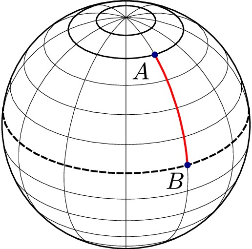
Image credit: Vikash Mittal - Geometric phase and its applications: topological phases, quantum walks and non-inertial quantum systems (FIGURE 2).
The shortest path between two points on a curved surface - a generalization of the concept of a "straight line" to curved geometry. On a flat plane a geodesic is just a straight line; on the surface of a sphere, geodesics are arcs of great circles; on more complex curved surfaces they can bend and twist while still remaining locally "as straight as possible" at every point.
Related terms:
- Great circle - the specific case of a geodesic on the surface of a sphere, formed by a plane passing through the sphere's center.
- Geodesic curvature - measure of how far a curve on a surface deviates from being a geodesic.
- Geodesic dome - structure whose triangulated struts approximate geodesic arcs across a sphere.
Articles:

Note
Related to geodesics, Platonic solids, and polyhedra.
Spherical shell structure of triangular struts whose vertices all lie on a circumscribed sphere. It's typically derived from a Platonic solid with triangular faces (usually an icosahedron) by subdividing each face some number of times (the dome's "frequency") and projecting the new vertices onto the sphere - higher frequencies mean more, smaller struts and a closer approximation of a sphere.
Named for the geodesic - the shortest path between two points on a curved surface - since its edges approximate great-circle arcs. The shell distributes structural stress evenly, giving it a high strength-to-weight ratio. Popularized (though not invented) by Buckminster Fuller, whose name was later borrowed for the similarly-shaped carbon molecules called buckminsterfullerenes.
Key terms:
- Geodesic - generalization of a straight line to curved surfaces; the shortest path between two points on the surface.
- Geodesic polyhedron - convex polyhedron made of triangles, usually derived from subdividing a Platonic or other simple polyhedron and projecting the vertices onto a sphere.
- Frequency - the number of times each face of the base polyhedron is subdivided before projection onto the sphere; written as
nV(e.g.3V), where a higher number means smaller, more numerous struts. - Strut - a single structural member (edge) connecting two vertices of the dome.
- Chord factor - ratio used to calculate the length of a given strut relative to the radius of the sphere.
Articles:
- Geodesic Domes by the Buckminster Fuller Institute
- Geodesic dome on Wikipedia
- Geodesic polyhedron on Wikipedia
- Explaining Dome Frequency by Domerama
- Geodesic Dome on Wolfram MathWorld
Notable software:
- Domerama calculators - strut-length and cover-pattern calculators for domes of various frequencies
Notable real-world geodesic domes:
- Climatron at the Missouri Botanical Garden in St. Louis, MO, USA. Diameter = 42m (138ft).
- La Géode at the City of Science and Industry in Paris, France. Diameter = 36m (118ft).
- Long Beach Cruise Terminal (formerly The Spruce Goose Dome) in Long Beach, CA, USA. Diameter = 122m (400ft).
- Matrimandir in Bommayapalayam, India. The building structure is a geodesic dome covered in golden discs. Diameter = 36m (118ft).
- Montreal Biosphere in Montreal, Québec, Canada. Designed by Buckminster Fuller himself in 1967. Diameter = 76m (249ft) .
- Science World building in Vancouver, Canada.
- Spaceship Earth in the EPCOT theme park at Walt Disney World in Orlando, FL, USA. Diameter = 50m (165ft).
- The Eden Project in Cornwall, England. Features multiple domes merged together into large, multi-area buildings.
- The Desert Dome at the Henry Doorly Zoo and Aquarium in Omaha, NE, USA. Diameter = 70m (230 ft).

Note
Related to the golden ratio and phyllotaxis.
Radial version of the golden ratio. It is the smaller of the two angles created by sectioning the circumference of a circle according to the golden ratio; that is, into two arcs such that the ratio of the length of the smaller arc to the length of the larger arc is the same as the ratio of the length of the larger arc to the full circumference of the circle.
In degrees the angle is approximately 137.5077640500 ..., or just 137.5 for brevity.
Articles:
- Golden angle on Wikipedia
- The Golden Angle by Go Figure
Creative projects:
- Golden Angle sculpture series by John Edmark

Note
Related to the Fibonacci sequence.
Also expressed as the Greek letter phi (φ), this irrational number pops up when the ratio of two numbers is the same as the ratio of their sum to the largest of the two numbers. It has been observed in many fields of the natural sciences at every scale and is has become associated with aesthetic beauty, giving it a nearly mythic reputation for some.
| Expressed algebraicly | |
| Expressed as line segments |  |
Articles:
- Golden ratio on Wikipedia
- Golden Ratio on Math is Fun
- Golden Ratio on Wolfram MathWorld

A surface defined by an equation in the form of 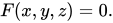
Examples of implicit surface equations:
| Plane | |
| Sphere | |
| Torus | |
| Surface of genus 2 | |
| Surface of revolution |
Articles:
- Implicit surface on Wikipedia
- Implicit surfaces by Paul Bourke
- Implicit surface a.k.a (signed) distance field: definition by Rodolphe Vaillant
Notable software:

Equations used to calaculate the positions of a series of rigidly-linked segments (called the kinematic chain) based on the location of the end effector, usually located at the tip of the last segment. Useful for robotic systems like drawing machines, robot arms, and more.
Inverse kinematics calculate the angles of each linked segment given the desired location of the end effector. Will give you the angles of each segment, which can in turn be converted into motor positions for a robot.
Forward kinematics calculate the location of the end effector given the angles and lengths of each linked segment.
Articles:
- Kinematics on Wikipedia
- Inverse kinematics on Wikipedia
- Forward kinematics on Wikipedia
Videos:
- Coding Challenge #64.1: Forward Kinematics by Daniel Shiffman
- Coding Challenge #64.2: Inverse Kinematics b Daniel Shiffman
- Coding Challenge #64.3: Inverse Kinematics - Fixed Point by Daniel Shiffman
- Coding Challenge #64.4: Inverse Kinematics - Multiple by Daniel Shiffman

Note
Related to DLA, DBM, Saffman–Taylor instability, reaction-diffusion, minimal surface, fluid simulation, and Laplace transform.
The Laplace equation,
That abstractness is exactly why it matters for morphogenesis: several branching growth patterns already covered elsewhere in this list are, mathematically, the same equation wearing different clothes - a family of processes collectively known as Laplacian growth.
Laplacian growth - from equation to organic form:
Each of these solves the Laplace equation in the region around a growing cluster, then advances the cluster's boundary fastest wherever the resulting field's gradient is steepest:
- Diffusion-limited aggregation (DLA) - random walkers stick where they first touch the cluster. In the continuum limit, the probability of a walker arriving at any boundary point is proportional to the gradient of the harmonic concentration field around the cluster - DLA is the stochastic, particle-based way of sampling a Laplacian growth process.
- Dielectric breakdown model (DBM) - solves the Laplace equation directly for an electric potential field around the growing discharge, then grows each boundary point in proportion to the local field gradient raised to a tunable power - the same idea as DLA, made explicit and continuous.
- Saffman–Taylor instability (viscous fingering) - inside a Hele-Shaw cell, the fluid pressure field obeys the Laplace equation (via Darcy's law), and the identical "grow fastest where the gradient is steepest" feedback produces the same branching, finger-like interface.
This is why DLA clusters, electrical discharge patterns, and viscous fingers all look so similar despite arising from unrelated physics - they're all boundaries growing into a harmonic field, differing only in their noise and boundary conditions.
Key terms:
- Laplacian operator (
$\nabla^2$ or$\Delta$ ) - the divergence of the gradient; measures how much a point's value differs from the average of its immediate surroundings. - Harmonic function - any solution to the Laplace equation; has no local maxima or minima except at the domain's boundary (the "mean value property").
- Poisson equation - the Laplace equation with a source term (
$\nabla^2 \varphi = f$ ); used whenever the field being solved has "generators" (charge, heat sources, image gradients) rather than being purely diffusive. - Boundary conditions - since the Laplace equation alone has infinitely many solutions, a specific field is picked out by fixing its values (Dirichlet) or its gradient (Neumann) on the domain's boundary - the growing cluster's surface, in Laplacian growth models.
- Laplacian growth - the general term for a growth process where the interface advances in proportion to the gradient of a harmonic field solved in the region ahead of it.
- Laplacian smoothing (mesh relaxation) - the discrete, iterative graphics technique of averaging each mesh vertex with its neighbors; converges toward a discrete solution of the Laplace equation.
Articles:
- Laplace's equation on Wikipedia
- Harmonic function on Wikipedia
- Laplacian smoothing on Wikipedia
- Fast Simulation of Laplacian Growth (PDF) by Theodore Kim et al. Academic review connecting DLA, dielectric breakdown, and viscous fingering as a single family of processes
- Discrete Differential Geometry: An Applied Introduction by Keenan Crane - course notes covering the discrete Laplacian as "the Swiss army knife of geometry processing," including mesh smoothing
Videos:
- Harmonic Functions from Khan Academy - short, visual introduction to the Laplacian and harmonic functions
Code projects:
- geometry-processing-smoothing by Alec Jacobson - reference implementation of Laplacian mesh smoothing from a geometry processing course
Note
Related to Laplace equation
Mathematical transform that converts a function of time into a function of complex frequency, turning differential equations into algebraic ones that are often easier to solve. It is widely used in engineering, physics, and control theory to analyze dynamic systems and their stability, resonance, and response.
The Laplace transform maps a time-domain function
Definition:
Where
Key properties:
| Property | Formula | Description |
|---|---|---|
| Linearity | Sum transforms equal sum of transforms | |
| Differentiation rule | Converts derivatives to algebraic operations | |
| Integration rule | Converts integrals to division by |
|
| Convolution theorem | Converts convolution to multiplication | |
| Final value theorem | Determines steady-state behavior | |
| Initial value theorem | Determines initial conditions | |
| Frequency shifting | Scaling exponential shifts frequency | |
| Time shifting | Delay in time domain multiplies by |
Key terms:
- Region of convergence (ROC) - the set of complex
$s$ values for which the Laplace integral converges - Pole - a value of
$s$ where$F(s)$ becomes infinite; poles determine system stability and response characteristics - Zero - a value of
$s$ where$F(s)$ equals zero - Transfer function - the Laplace transform of a system's impulse response; describes how a system responds to inputs
- Inverse Laplace transform - converting from frequency domain back to time domain; often done via partial fraction decomposition
- Partial fraction decomposition - breaking a complex rational function into simpler fractions to facilitate inverse transformation
Articles:
- Laplace transform on Wikipedia
- Laplace Transform on Wolfram MathWorld
- Laplace Transform Tables and Properties by Paul's Online Math Notes
- Introduction to the Laplace Transform from MIT OpenCourseWare (differential equations course)
Also known as Bowditch curves, these figures plot the trajectories of a point as it follows the path of two simultaneous sinusoidal motions.
Can be created using various physical systems including oscilloscopes, harmonographs, and more.
Equations:
Articles:
- Lissajous curve on Wikipedia
- Lissajous curve from MathCurve
- Lissajous Curves from DataGenetics
Videos:
- Coding Challenge #116: Lissajous Curve Table by Daniel Shiffman (Github repo with source code for p5.js and Processing)
- #48: Basics of Lissajous Patterns on an Oscilloscope by w2aew

Note
Related to soft-body physics, cloth simulation, Verlet physics, and physics engines.
A mass-spring system is a general mathematical model for deformable bodies: a graph of point masses connected by springs that obey Hooke's law (restoring force proportional to displacement from a rest length). It's one of the oldest and most widely reused abstractions in computational physics, showing up not just in computer graphics but in structural engineering (truss analysis), molecular dynamics (bond modeling), and biomechanics (tissue and muscle models). Its appeal is that a small number of local rules - distance constraints and simple forces - can produce believable global deformation without solving a full continuum mechanics problem.
In graphics and simulation, mass-spring systems are the conceptual backbone of cloth simulation, rope/hair simulation, and soft-body deformation, and are typically stepped forward with Verlet integration for stability. Real-time applications commonly layer three kinds of springs to control different deformation modes: structural springs (resist stretching), shear springs (resist skewing), and bend springs (resist folding).
Algorithm at a glance:
* indicates a potential simulation parameter
- Represent the body as a graph of point masses, each with position, velocity, and mass*.
- Connect masses with springs, each with a rest length and stiffness*.
- For each spring, compute the restoring force:
F = stiffness × (current_distance - rest_length). - Add a damping force proportional to relative velocity*:
F_damping = damping × relative_velocity. - Sum spring, damping, and external forces (gravity, wind, etc) on each mass.
- Integrate mass positions forward, commonly with Verlet integration.
- Detect and resolve collisions with rigid bodies and self-collisions.
- Repeat until the system settles or the simulation ends.
Key terms:
- Hooke's law - the restoring force in a spring is proportional to its displacement from rest length, scaled by a stiffness constant.
- Rest length - the preferred distance between two connected masses; springs pull toward this distance.
- Stiffness (spring constant) - how strongly a spring resists stretching; higher values resist deformation more.
- Damping - dissipative force proportional to velocity; prevents infinite oscillation and lets systems settle.
- Structural constraints - springs between nearest neighbors; define topology and resist stretching.
- Shear constraints - diagonal springs between diagonal neighbors; resist skewing.
- Bend constraints - springs between masses separated by one neighbor; resist folding/creasing.
Articles:
- Mass-Spring Model - interactive visualization of spring-mass dynamics
- Advanced Character Physics by Thomas Jakobsen - the classic paper connecting Verlet integration to mass-spring constraint systems
- Real Time Simulation of Soft Objects Using Mass-Spring System (PDF) - academic paper on soft-body simulation
Code projects:
- Rope Simulation (CS184 Discussion) - basic rope/cloth mass-spring implementation
- Cloth Simulation - interactive cloth simulator demonstrating mass-spring constraints
- Mass-Spring System for Soft-Body Simulation - 3D soft-body physics implementation
Videos:
- Coding Challenge #26: Spring Physics by The Coding Train - implementing mass-spring systems in p5.js

The medial axis is sort of like the "skeleton" of a shape. It consists of a set of lines and curves upon which every point is equidistant between at least one closest point on the shape's boundary. In 2D this skeleton can also be thought of as a set of lines/curves whose points are the centers of circles that are tangent to at least two points on the shape's boundary.
Has applications in computer vision, pose estimation, 2D/3D character rigging, architecture, BIM (escape route optimization), and more.
Related terms:
- Medial-axis transform - medial axis together with the associated radius function of the maximally inscribed discs. Can be used to reconstruct a shape.
- Topological Skeleton
- Straight skeleton - similar to medial, except always is made up of straight line segments whereas medial axis may contain curves.
- Scale Axis Transform - generalization of medial axis transform
Articles:
- Medial axis on Wikipedia
- "A transformation for extracting new descriptors of shape" by Henry Blum
Notable Tools:
- Skeleton-Tracing, a code library for computing topological skeletons as a set of polylines from binary images. Provides implementations in C, C++, Java, JavaScript, Python, Go, C#/Unity, Swift, Rust, Julia, Processing, and OpenFrameworks.

Note
Related to Laplace equation.
A minimal surface is a surface that locally minimizes area, which means it settles into the smallest possible shape for a given boundary while keeping its mean curvature equal to zero. Minimal surfaces show up in architecture, material design, geometry, and optimization, and they are useful whenever you want a smooth surface or membrane that uses as little area as possible.
A soap film stretched across a wire frame is the classic physical example: the film naturally relaxes into a shape that balances tension everywhere. Frei Otto's soap-bubble experiments were important for showing how these forms emerge in the real world.
Equations:
| Equation | Explanation |
|---|---|
|
Where: |
The minimal surface condition says the average of the principal curvatures is zero. |
|
Where: |
The minimal surface equation is the graph form of a minimal surface. |
|
Where: |
The area functional gives the total surface area. |
Key terms:
- Area functional - the integral that gives the total area of a surface
- Mean curvature - the average of the two principal curvatures at a point on a surface
- Minimal surface equation - the differential equation whose graph solutions are minimal surfaces
- Minimal surface condition - the equation
$H = 0$ that defines a minimal surface - Plateau's problem - finding the least-area surface spanning a given boundary
- Principal curvatures - the two main curvatures of a surface at a point, measured in perpendicular directions
Examples:
| Term | Equation |
|---|---|
| Catenoid | |
| Helicoid | |
| Gyroid |
Articles:
- Minimal surface on Wikipedia
- Plateau's problem on Wikipedia
- Constant mean curvature (CMC) surface on Wikipedia
Notable software:
- Surface Evolver by Ken Brakke - interactive software for minimizing surface energies and constraints
- Kangaroo Physics - Grasshopper plugin for physics-based form-finding and constraint solving, extensively used for minimal surface and structural exploration
- PufferFish - Grasshopper plugin with mathematical surface components for minimal surface visualization and manipulation
- Houdini Vellum - constraint-based cloth and hair solver useful for simulating membrane and fabric-like minimal surface behavior
- MinimalSurface addon - Blender addon specifically designed for finding and generating minimal surfaces with prescribed boundary conditions
- Mathematica Implicit Surface Visualization - tools for rendering and analyzing implicit surface equations including minimal surfaces
Notable creative work:
- Frei Otto's soap-bubble form-finding studies
- Bathsheba Grossman - metal sculptures and mathematical artworks
- Rinus Roelofs - sculptures and installations
Notable real-world buildings:
- Olympiastadion (Munich, Germany) by Günther Behnisch and Frei Otto
- Multihalle Mannheim (Munich, Germany)
- German Pavilion at Expo 67 (Montreal, Canada) by Frei Otto and Rolf Gutbrod
Natural phenomena:
- Soap bubbles and soap films - the classic physical analog for minimal surfaces
- Butterfly wings (Papilio palinurus) - gyroid structure in wing scale ridges creates structural color via photonic crystal effects
- Weevil exoskeleton (Lamprocyphus augustus) - Schwarz-D (diamond-type TPMS) surface with photonic properties
- Sea urchin skeleton (echinoderm stereom) - diamond-type minimal surface formed from single-crystal magnesian calcite; guided by cytoskeletal templating
- Endoplasmic reticulum - bicontinuous membrane network with negative Gaussian curvature and minimal surface-like topology
- Mitochondrial cristae - morphology accurately predicted by minimal surface models; structure adapts based on cell energy state
- Block copolymers (e.g., PS-b-PEO) - self-assemble into gyroid phase with bicontinuous nanochannels
- Bicontinuous lipid cubic phases (monoolein/water) - form gyroid, diamond, or primitive TPMS depending on hydration level; used in drug delivery and protein crystallization

Class of optimization problems that involve determining efficient ways to arrange (pack) objects into containers. Packing problems can be tackled using discrete mathematical methods, physics systems (as seen in Nervous System's Kinematics series), and even genetic algorithms and machine learning.
Has major applications in digital fabrication, manufacturing, and shipping logistics where material and space usage is directly related to costs. In 2D, packing/nesting problem solutions are useful for minimizing waste material in sheet goods like plywood and sheet steel, even for hobbyists. In 3D these solutions are useful for fitting as many objects as possible into 3D printer build envelopes (see article from Sculpteo).
Related terms:
Articles:
- Packing problems on Wikipedia
- Random space filling of the plane by Paul Bourke
- Optimal Packing from Data Genetics
- Circle Packing on Wolfram MathWorld
- Bin packing problem on Wikipedia
- Sphere packing on Wikipedia
- Close-packing of equal spheres on Wikipedia
- Packing Problems - collection of papers by Ernesto Birgin and collaborators
Notable tools:
Videos:
- Coding Challenge #50.1: Animated Circle Packing - Part 1 by Daniel Shiffman

Mathematical framework that studies the behavior of connected clusters in random networks. At its core, percolation explores the threshold at which a system transitions from isolated fragments to a connected network spanning the entire space - a critical phenomenon with applications in material science, epidemiology, network analysis, and growth simulation.
The classical model places sites or bonds randomly on a grid, each with some occupation probability
Key concepts:
- Percolation threshold (
$p_c$ ) - the occupation probability at which a spanning cluster first appears. The value depends on the lattice type: for square lattices$p_c \approx 0.593$ (bond) or$0.589$ (site), for triangular lattices$p_c \approx 0.5$ (bond), etc. - Cluster - a connected group of occupied sites or bonds.
- Giant component - the largest, system-spanning cluster that emerges above the threshold.
- Lattice types - square, triangular, hexagonal, random graphs, and others; each has different percolation thresholds and scaling behavior.
- Major models:
- Bond (Bernoulli) percolation - bonds (edges) between fixed sites are randomly occupied; relates to fluid flow through porous media.
- Site percolation - individual sites (nodes) are randomly occupied; relates to disease spread or forest fire models.
- Mixed percolation - combines site and bond percolation in one model, requiring both the sites and the bonds connecting them to be open for a cluster to form.
- Bootstrap percolation - starting from a random set of occupied sites, empty sites are iteratively "infected" once they have at least
$k$ occupied neighbors, repeating until no more sites change; models cascading activation like infection spread or social contagion. - Inhomogeneous percolation - the occupation probability
$p$ varies from site to site (or bond to bond) instead of being uniform, e.g. to model spatially-varying material properties. - Long-range percolation - bonds can connect any two sites, not just nearest neighbors, with connection probability typically decaying with distance (often as a power law); can percolate via rare long "jumps" even below the classical threshold.
- Directed percolation (oriented percolation) - bonds/sites can only be traversed along a preferred direction (e.g. "downward" through time); models epidemic spreading and non-equilibrium phase transitions.
- Continuum percolation - occupation is defined over continuous space rather than a discrete lattice, e.g. overlapping disks or spheres; models material conductivity and wireless network coverage.
- Germ-grain model - general stochastic-geometry framework of "germs" (points) dressed with "grains" (shapes) that may be correlated with one another or their surroundings.
- Boolean model (Poisson Boolean model) - the germ-grain model's independent special case: germs scattered via a Poisson process, each dressed with an independent random grain; percolation occurs when grains overlap into a spanning cluster.
- Disk model (Gilbert disk model) - special case of the Boolean model where every grain is a disk of fixed or random radius; used for random geometric graphs and wireless/sensor network connectivity.
- Random-connection model - generalizes the Boolean/disk model into a random graph: any two points connect with a probability given by a distance-dependent "connection function," rather than by fixed-radius grain overlap.
- Invasion percolation - growth advances by always occupying the weakest/most accessible available site rather than a random one; models fluid displacement in porous media.
- First-passage percolation - instead of open/closed sites or bonds, each bond is assigned a random "passage time"; studies how quickly a fluid spreads from a source along the fastest weighted paths, producing random growth shapes.
- Random-cluster model (Fortuin–Kasteleyn model) - generalizes percolation with an extra parameter
$q$ that continuously interpolates between percolation ($q=1$ ), the Ising model ($q=2$ ), and the Potts model ($q>2$ ).
- Critical exponents - power-law relationships describing cluster size distribution, correlation length, and other properties near
$p_c$ . These exponents are universal across many percolation models. - Universality class - percolation models grouped by shared critical exponent values; a hallmark of statistical physics.
Percolation can model porous media (oil migration through rock), disease spread (how infections propagate through a population), forest fires (how rapidly fires spread through dense vegetation), and network robustness (how many nodes can fail before connectivity is lost). In the context of morphogenesis, percolation-based growth can generate branching patterns, fragmented structures, and networks with natural-looking interconnectivity.
Articles:
- Percolation theory on Wikipedia
- Percolation by Paul Bourke
- Percolation Threshold on Wolfram MathWorld
Code projects and interactive tools:
- “Barista's Secret”: Percolation on a lattice by Dirk Brockmann - interactive visualization of site percolation on a square lattice
- Red Blob Games - Percolation - explores percolation on different grid types (mentions percolation effects in hexagonal grids)

Note
Related topics include the golden ratio, the golden angle, and the Fibonacci sequence.
Refers to the arrangement (taxis) of leaves (phyllo) on a plant stem. Also can refer to seed arrangements and succulent geometry.
Types:
- Opposite - two leaves arise from the stem at the same level on opposite sides of the stem
- Alternate - each leaf arises at a different point (node) on the stem
- Whorled - arrangement of leaves that radiate from a single point and surround or wrap around the stem, as seen in the thumbnail for this section.
- Distichous - special case of either opposite or alternate leaf arrangement where the leaves on a stem are arranged in two vertical columns on opposite sides of the stem
- Decussate - occurs when successsive pairs of leaves arranged in the opposite pattern are 90 degrees apart, as in Aizoaceae family
Articles:
- Phyllotaxis on Wikipedia
- Chapter 4: Phyllotaxis from Algorithmic Botany book
- Phyllotaxis on Wolfram MathWorld
Code projects:
- ofxPhyllotaxis by Davide Prati (edap)
Videos:
- Coding Challenge #30: Phyllotaxis by Daniel Shiffman

Note
Related to polyhedra and Archimedean solids.
Set of regular, convex polyhedra constructed using congruent, regular polygonal faces with the same number of faces meeting at each vertex. Euclid (and perhaps Theaetetus proved mathematically that there are only five shapes that fit this criteria (below).
| Name | Polygon type | Faces | Edges | Vertices | Image |
|---|---|---|---|---|---|
| Tetrahedron | Triangle | 4 | 6 | 4 |  |
| Cube | Square | 6 | 12 | 8 |  |
| Octahedron | Triangle | 8 | 12 | 6 |  |
| Dodecahedron | Pentagon | 12 | 30 | 20 |  |
| Icosahedron | Triangle | 20 | 30 | 12 |  |
Articles:
- Platonic solid on Wikipedia
- Platonic Solids on Tutors.com
Videos:
- 5 Platonic Solids by Numberphile

Note
Related to Platonic solids, Archimedean solids, geodesic domes, and Conway operators.
A polyhedron is a solid bounded by flat polygonal faces, straight edges, and sharp vertices - the Platonic and Archimedean solids are just the two best-known families in a much larger space of shapes. For generative artists, polyhedra are a useful design space precisely because they're so constrained: a handful of construction rules (regular faces, identical vertices, symmetric arrangements) generate a finite, well-catalogued set of "correct-looking" forms, which is why the same few solids keep reappearing as base meshes for subdivision, geodesic domes, and procedural modeling more broadly.
Key concepts:
- Convex vs. concave - convex polyhedra bulge outward everywhere with no self-intersections; concave ones have indentations or intersecting faces.
- Classes - groupings based on construction rules, e.g. Platonic, Archimedean, Catalan, Kepler-Poinsot, Johnson, prisms/antiprisms, and near-misses.
- Symmetry - when a shape can be rotated or reflected and still look exactly the same.
- Stellation and facetting - dual operations for making new polyhedra from old ones: stellation extends face planes outward; facetting cuts new faces from existing vertices.
Major classes:
- Platonic solids - the 5 regular convex polyhedra; one type of regular polygon face, identical arrangement at every vertex.
- Archimedean solids - 13 semi-regular convex polyhedra with two or more types of regular polygon faces meeting identically at every vertex.
- Catalan solids - the 13 duals of the Archimedean solids; face-transitive rather than vertex-transitive, so their faces aren't regular polygons but their vertex figures are.
- Kepler-Poinsot solids - the 4 regular star polyhedra (small/great stellated dodecahedron, great dodecahedron, great icosahedron); self-intersecting stellations or facettings of the dodecahedron and icosahedron.
- Johnson solids - the 92 remaining convex solids with regular polygon faces that aren't vertex-transitive (i.e. everything left once Platonic, Archimedean, prisms, and antiprisms are excluded).
- Prisms and antiprisms - two infinite families of uniform polyhedra: two parallel n-gon faces connected by a ring of squares (prism) or triangles (antiprism).
- Near-misses - convex solids with faces so close to regular that they read as "correct" at a glance (e.g. the soccer-ball-style truncated icosahedron variants used in geodesic-adjacent design); popular in architecture and fabrication because slightly irregular faces can simplify paneling or tiling.
Symmetry:
A shape has symmetry when it can be rotated or reflected and still look exactly the same - spin a cube 90° around an axis through two opposite faces and you can't tell it moved. The full set of ways a shape can do this is called its symmetry group, and the larger it is, the more interchangeable the shape's faces, edges, and vertices look.
Highly symmetric polyhedra fall into just three of these groups (doubled again with mirror reflections) - part of why the same few base shapes keep recurring in generative work:
- Tetrahedral symmetry - 12 rotations (24 with reflections); the symmetry of the tetrahedron.
- Octahedral symmetry - 24 rotations (48 with reflections); shared by the cube and octahedron since they're duals of each other.
- Icosahedral symmetry - 60 rotations (120 with reflections); shared by the dodecahedron and icosahedron, and the reason icosahedral subdivision is the standard approach for geodesic domes.
A polyhedron's symmetry group also determines whether every vertex looks like every other vertex (isogonal, true of the Platonic and Archimedean solids), every face looks like every other face (isohedral, true of the Platonic and Catalan solids), or every edge looks like every other edge (isotoxal).
Stellation and facetting:
These are dual, opposite operations for generating new polyhedra from existing ones:
- Stellation - extending a polyhedron's face planes outward until they intersect each other again, producing a larger, usually self-intersecting shape. The four Kepler-Poinsot solids are the only regular stellations of the dodecahedron and icosahedron, but a single seed shape (like the icosahedron) can have dozens of named stellations.
- Facetting - creating new faces using only a polyhedron's existing vertices, without adding any new ones - effectively "cutting into" the solid rather than extending outward.
Key terms:
- Face, edge, vertex - the three basic elements of a polyhedron.
- Euler's formula -
V - E + F = 2for any simple convex polyhedron; a quick sanity check for procedurally generated meshes. - Dual polyhedron - swapping faces and vertices produces a shape's dual (cube ↔ octahedron, dodecahedron ↔ icosahedron, tetrahedron ↔ itself).
- Uniform polyhedron - vertex-transitive with regular polygon faces; covers the Platonic and Archimedean solids, prisms, antiprisms, and their non-convex "star" counterparts.
- Schläfli symbol - shorthand
{p, q}describing a regular polyhedron by its face polygon (p-gon) and how many meet at each vertex (q); star polyhedra use fractions, e.g.{5/2, 5}for the small stellated dodecahedron. - Vertex figure - the cross-section shape formed by slicing off a vertex; used to classify uniform polyhedra by which polygons meet there.
- Convex hull - the smallest convex shape enclosing a set of points; a common generative technique for deriving a convex polyhedron from a symmetric point distribution.
Articles:
- Polyhedron on Wikipedia
- Point groups in three dimensions on Wikipedia - overview of the tetrahedral, octahedral, and icosahedral symmetry groups
- Stellation on Wikipedia
- Faceting on Wikipedia
- Stellations by George Hart - short illustrated explanation of the stellation process
- Visual Polyhedra by David McCooey - interactive 3D models organized by class (Platonic, Archimedean, Catalan, Kepler-Poinsot, Johnson, and more), with downloadable geometry data
- Virtual Polyhedra: The Encyclopedia of Polyhedra by George Hart
Videos:
- Kepler-Poinsot Polyhedra - overview of the four regular star polyhedra
Notable tools:
- Stella by Robert Webb - dedicated polyhedra exploration software (Great Stella, Small Stella, Stella4D) supporting stellation, facetting, augmentation, dualization, convex hulls, and printable nets
- Antiprism by Adrian Rossiter - open-source command-line toolkit for generating, transforming, and converting polyhedra (GitHub)
- Polyhedronisme by Anselm Levskaya - web app for building polyhedra from a seed shape using Conway polyhedron notation operators
Code projects:
- polyhedronisme - source code for the Conway-notation polyhedron builder above
- PolyJS (GitHub) by Matthew Arcus - generates and animates uniform polyhedra and compounds in Three.js using the Wythoff construction
- Polyhedra (Three.js) by Lee Stemkoski - renders polyhedra using vertex/face data from George Hart's polyhedra encyclopedia

Note
Related to DBM, DLA, differential growth, reaction-diffusion, fluid simulation, Hele-Shaw cells, and Laplace equation
Also known as viscous fingering, this is a fluid dynamics instability that occurs at the interface between two fluids of different viscosity when a less viscous fluid is pushed into a more viscous one - inside a narrow gap such as a Hele-Shaw cell, or through a porous medium. Rather than advancing as a flat front, the interface spontaneously breaks up into branching, finger-like intrusions.
The instability is a positive feedback loop: any small bump that forms on the interface sits in a region of lower flow resistance, so it advances faster than its surroundings, growing further ahead and widening into a finger; the same feedback then acts along the flanks of that finger, splitting its tip and producing a branching structure reminiscent of diffusion-limited aggregation and the dielectric breakdown model. Interfacial tension between the two fluids counteracts this, damping out short-wavelength wrinkles and setting a characteristic finger width - the balance between the two effects selects the fairly regular finger spacing seen in real experiments.
Key terms:
- Viscous fingering - the common, descriptive name for the same phenomenon.
- Mobility ratio - ratio between the two fluids' viscosities (or, in a porous medium, permeabilities); the interface is unstable only when the injected fluid is less viscous than the fluid it displaces.
- Hele-Shaw flow - the mathematical description of flow through the thin gap of a Hele-Shaw cell, from which the instability was originally derived.
- Interfacial (surface) tension - force resisting curvature of the interface; suppresses high-frequency wrinkles and sets a preferred finger width/wavelength.
- Tip-splitting - the process by which a growing finger becomes unstable at its own tip and divides into two smaller fingers, driving the fractal branching seen in the radial configuration.
- Channel vs. radial geometry - the two most common experimental setups: injection along a straight channel typically produces one dominant "Saffman–Taylor finger," while injection from a central point (radial) produces repeated tip-splitting into many fingers.
DIY experiments:
Viscous fingering can be observed with everyday materials without specialized equipment. When two surfaces are slowly peeled or pulled apart with a thin viscous layer (honey, jam, corn syrup, or hand lotion) between them, the less viscous fluid (air) displaces the viscous layer, creating fingerlike flow patterns at the retreating interface. The same effect occurs in setups such as:
- Slowly peeling apart two wet pieces of paper
- Separating two wet glass plates or acrylic sheets
- Pulling apart plastic wrap or film from a surface coated with a viscous substance
- Lifting a glass plate from a table with a thin layer of honey, oil, or gel underneath
These "peeling" setups exhibit viscous fingering because the viscous fluid resists the air's advance, creating an unstable interface that spontaneously breaks into fingers. This is closely related to the lifted Hele-Shaw cell concept—in both cases, viscous resistance shapes fluid interfaces during separation or displacement, revealing the same underlying physics.
Articles:
- Saffman–Taylor instability on Wikipedia
- The penetration of a fluid into a porous medium or Hele-Shaw cell containing a more viscous liquid (1958) by Philip Saffman and G. I. Taylor. The original paper.
- Viscous Fingering in Porous Media (1987) by G. M. Homsy. Widely-cited review of the phenomenon.

Note
Related to Fourier series
Spherical harmonics are a set of special functions defined on the surface of a sphere that form a complete, orthonormal basis - meaning any reasonably well-behaved function over the sphere (e.g. a bumpy radius, a lighting environment, a temperature field) can be reconstructed as a weighted sum of them, in the same way a Fourier series reconstructs a periodic signal from sines and cosines. They arise naturally as the angular part of the solution to Laplace's equation in spherical coordinates, which is why they show up throughout physics wherever spherical symmetry is involved - gravitational and electric potentials, atomic orbitals, geodesy, and the cosmic microwave background.
Each spherical harmonic is indexed by a degree
Key terms:
- Degree (
$l$ ) and order ($m$ ) - indices identifying each spherical harmonic; the degree controls how many nodal lines (angular frequency) a harmonic has, while the order controls their orientation around the polar axis. - Legendre polynomials (and associated Legendre functions) - the family of functions used to build the latitude (polar-angle) part of each spherical harmonic.
- Real vs. complex spherical harmonics - two equivalent bases for the same functions; real harmonics are more common in graphics and engineering, complex ones in quantum mechanics.
- Multipole expansion - representing a field (gravitational, electric, etc.) as a sum of spherical harmonics weighted by coefficients, ordered from coarse (monopole/dipole) to fine detail.
- Precomputed radiance transfer (PRT) - computer graphics technique that stores lighting/shading information as a small set of spherical harmonic coefficients for fast, approximate real-time rendering.
- SPHARM (spherical harmonic shape description) - representing an arbitrary closed 3D surface, such as an organic blob or biological structure, as a set of spherical harmonic coefficients; used for shape analysis, comparison, and generative modeling.
Articles:
- Spherical harmonics on Wikipedia
- Spherical Harmonics by Paul Bourke
Code projects and tools:
- google/spherical-harmonics (C++) - graphics-oriented library for evaluating, projecting, and rotating spherical harmonic basis functions, including diffuse irradiance/environment lighting helpers.
- SHTOOLS/SHTOOLS (Fortran 95 / Python,
pyshtools) - library for spherical harmonic transforms, spectral analysis, and working with gravity/magnetic/topography field data. - A Symphony of Spheres: Animating Spherical Harmonics in Blender with Python and Shape Keys by Ben de Vries

Trajectories of deterministic dynamical systems that exhibit chaotic behavior while remaining confined within a bounded region of space. Unlike ordinary attractors (fixed points or periodic cycles), strange attractors have a fractal structure with infinite detail and display sensitive dependence on initial conditions - tiny differences in starting state lead to wildly divergent outcomes. Despite their deterministic rules, the long-term behavior appears random or turbulent.
Strange attractors emerge in nonlinear systems where feedback loops create complex dynamics. They are "strange" because they combine order (the system never leaves a bounded region) with chaos (unpredictable behavior). They are "attractors" because trajectories from nearby initial conditions are pulled toward them over time. Their fractal dimension is typically non-integer, a hallmark of their geometric complexity.
Strange attractors have been observed in fluid dynamics (turbulence), weather systems (weather chaos), population dynamics, electronic circuits, and more. In generative art and morphogenesis, they are often used to create organic-looking, intricate patterns and forms that would be difficult or impossible to design by hand. The self-similar, fractal-like structures they produce can simulate natural phenomena like cloud formations, terrain, and biological branching patterns.
Key terms:
- Attractor - a set of states (points in phase space) toward which a dynamical system evolves, regardless of initial conditions. Non-strange attractors include fixed points and periodic orbits.
- Phase space - an abstract mathematical space where each point represents a possible state of the system; trajectories trace the system's evolution through this space.
- Chaos / Chaotic behavior - deterministic evolution that is sensitive to initial conditions; small perturbations grow exponentially, making long-term prediction impossible even though the system is not random.
- Sensitive dependence on initial conditions - the hallmark of chaos; trajectories starting arbitrarily close together diverge exponentially fast. Related to the concept of the Lyapunov exponent.
- Fractal structure - strange attractors typically have infinite detail at all scales, with a non-integer (fractal) dimension.
- Basin of attraction - the set of initial conditions from which trajectories are drawn to a particular attractor.
- Bifurcation - a qualitative change in system behavior as a parameter varies; can lead to onset of chaos or transition between different types of attractors.
Notable attractors:
- Clifford attractor
- Duffing attractor
- Hénon attractor
- Lorenz attractor
- Multiscroll attractor (a.k.a double-scroll attractor or Chua's attractor)
- Rössler attractor
Articles:
- Strange attractor section on Wikipedia article for attractors

Also known as the Lamé curve, this equation describes a closed curve that can generate shapes that look like pinched or inflated ellipses. At the extremes of the parameter space the shapes can range from an outline of a plus (+) symbol to a nearly rectangular shape with rounded corners.
Equations:
| General form | |
| Parametric |
Articles:
- Superellipse on Wikipedia
- Superellipse on Wolfram MathWorld
- Supershapes (Superformula) by Paul Bourke
Videos:
- Coding Challenge #23: 2D Supershapes by Daniel Shiffman (Github repo with Processing and p5.js code)

Generalized version of the superellipse formula proposed by Johan Giellis around 2000, capable of far more variety than the original superellipse. Unfortunately, Johan has patented use of the formula (via his company Genicap) in both the US and the EU, which means you should avoid using it for any kind of commercial work, or work that could be commercialized in some way later.
The superformula can be used to generate both 2D and 3D forms. To create 2D forms, use the general form equation to obtain polar coordinates that can be converted into Cartesian coordinates for drawing on a screen. To create 3D forms, compute the polar coordinates for two 2D supershapes, then "mix" them together using the 3D equations below.
Equations:
| General form | |
| 3D equations |
Where r is a radius and φ (phi) is an angle.
Where φ (latitude) varies between −π/2 and π/2 and θ (longitude) between −π and π.
Articles:
- Superformula on Wikipedia
- Supershapes / Superformula by Paul Bourke
Code projects:
- SuperformulaSVG-for-web by Jason Webb (Javascript, p5.js)
- SuperformulaSVG by Jason Webb (Processing)
- Visualize: Superformula from FORM+CODE book
- glsl-superformula by JC Leyba (Software)
- supershape.js by Sebastian Sadowski (ahoiin)
Videos:
- Coding Challenge #26: 3D Supershapes by Daniel Shiffman (Processing sketch on Github)

Note
Related to polyhedra, Wave Function Collapse (WFC), and Delaunay triangulation and Voronoi diagrams.
A tiling (or tessellation) is a covering of a plane, or other surface, by one or more shapes ("tiles") with no gaps and no overlaps. Like polyhedra, tilings are a design space defined by a small set of construction rules, which makes them a reliable source of "correct-looking" repeating patterns for generative art, procedural texture generation, and physical fabrication (laser-cut panels, tiled floors, quilting).
Key concepts:
- Periodic vs. aperiodic - periodic tilings repeat via simple translation, so a single finite patch can tile the whole plane; aperiodic tilings (like Penrose tilings) never repeat via translation alone, no matter how far you zoom out.
- Regular and semi-regular tilings - the 2D analog of Platonic and Archimedean solids: 3 regular tilings (one type of regular polygon) and 8 semi-regular tilings (2+ types), each with an identical arrangement of polygons at every vertex.
- Symmetry (wallpaper groups) - every repeating 2D pattern falls into one of exactly 17 wallpaper groups, based on which combination of translations, rotations, reflections, and glide reflections leave the pattern looking unchanged.
- Substitution tilings - built by repeatedly subdividing each tile into smaller copies of the same prototile set according to a fixed rule; many aperiodic tilings, including Penrose's, can be generated this way.
Notable named tilings:
- Penrose tiling - the best-known aperiodic tiling, built from just two prototiles (kite & dart, or two rhombi) related by the golden ratio.
- Wang tiles - square tiles with colored edges that must match their neighbors, with no rotation allowed in the original formalism; widely used in computer graphics for generating large, non-repetitive textures, height fields, and point distributions from a small tile set.
- Truchet tiles - simple square tiles (split diagonally, or decorated with quarter-circle arcs) that, placed in random orientations, produce intricate maze-like or flowing patterns; a long-running favorite in generative art, first described by Sébastien Truchet in 1704.
- The Hat and Spectre - the first known aperiodic monotiles ("einsteins"), discovered in 2023 by David Smith, Craig Kaplan, Joseph Myers, and Chaim Goodman-Strauss. Each forces aperiodicity using a single tile shape and no matching rules, resolving a problem that had been open since the 1960s.
- Isohedral (Escher-style) tilings - tilings where every tile is equivalent to every other tile under the pattern's symmetries; the class M.C. Escher's interlocking animal and figure tessellations belong to.
Key terms:
- Prototile - one of the shape(s) allowed in a tiling; a monotile is a tiling that uses just one.
- Edge-to-edge - a tiling where tiles only ever share a full edge with a neighbor, never a partial one.
- Vertex configuration - the cyclic sequence of polygon types meeting at a vertex, e.g.
3.6.3.6for a triangle-hexagon-triangle-hexagon arrangement. - Matching rules - markings or notches added to prototiles that forbid periodic arrangements; used by some, but not all, aperiodic tilings to enforce non-repetition.
Articles:
- Tessellation on Wikipedia
- Wallpaper group on Wikipedia
- Introductory Tiling Theory for Computer Graphics (PDF) by Craig S. Kaplan - concise academic introduction to tiling theory for a graphics/programming audience
- An aperiodic monotile (PDF) by David Smith, Joseph Samuel Myers, Craig S. Kaplan, and Chaim Goodman-Strauss - the original "Hat" paper
- The Hat and the Spectre from the National Museum of Mathematics - accessible overview of both 2023 discoveries
Videos:
- 5 and Penrose Tiling by Numberphile
- Aperiodic monotile animation featuring the discoverers of "the Hat"
Notable tools:
- Tactile.js by Craig Kaplan - JavaScript library for representing, manipulating, and drawing Escher-style isohedral tilings (C++ version)
- Pattern Collider by Aatish Bhatia - interactive web tool for exploring quasiperiodic tilings, including Penrose and the Hat/Spectre monotiles
- Penrose by Carnegie Mellon University - web-based tool that creates images from text notation. (Github repo)
Code projects:
- Penrose.js - pure JavaScript library for generating Penrose tilings, rendered to canvas or bitmap
- Pattern Collider - source code for the interactive tool above

Asks the question "Given a list of cities and the distances between each pair of cities, what is the shortest possible route that visits each city and returns to the origin city?" This classic problem is computer science classrooms to teach algorithm design and optimization techniques.
Useful for creating single-line drawings for use with pen plotters, laser cutters, CNC machines, and more.
Articles:
- Travelling salesman problem on Wikipedia
- Traveling Salesman Problem from Google OR-Tools
Notable software:
- StippleGen from Evil Mad Scientist Laboratories can calculate TSP paths.

Note
Related to physics engines and particle systems.
Image credit: Matthew Fisher - Cloth
Family of numerical integration methods for simulating motion that skip storing velocity explicitly, instead deriving it implicitly from a particle's current and previous position. Named after French physicist Loup Verlet, who used it for molecular dynamics simulations in the 1960s, though the technique dates back further.
At each step, a particle's next position is calculated from its current position, its previous position, and the acceleration currently acting on it:
newPosition = 2 * currentPosition - previousPosition + acceleration * timeStep^2
Because positions - not velocities - are what's being directly manipulated, distance constraints (like the fixed-length "sticks" connecting particles in a rope, cloth, or soft body) can be enforced by simply nudging connected particles toward or away from each other until the constraint is satisfied, without separately tracking or adjusting velocity. This makes Verlet integration especially popular for simulating chains, cloth, ragdolls, and other constraint-based systems in games, creative coding, and animation - and it forms the conceptual basis for the more general Position Based Dynamics approach used in many modern physics engines.
Key terms:
- Implicit velocity - since a particle's velocity is never stored directly, it can be recovered as the difference between its current and previous position.
- Distance constraint - a rule (often visualized as a "stick") requiring two particles to stay a certain distance apart; satisfied directly by moving positions rather than applying forces.
- Position Based Dynamics (PBD) - generalization of Verlet-style constraint solving into a broader framework for simulating cloth, rigid bodies, fluids, and more.
- Numerical stability - Verlet integration is more stable than simple Euler integration over long simulations, since it approximately conserves energy.
Articles:
- Verlet integration on Wikipedia
- Advanced Character Physics (PDF) by Thomas Jakobsen - classic, widely-cited article on using Verlet integration for constraint-based cloth and character simulation, developed for the game Hitman: Codename 47
- Ten Minute Physics by Matthias Müller - video tutorial series building from basic particle simulation up to Position Based Dynamics
- Verlet Physics with Toxiclibs.js chapter from Daniel Shiffman's Nature of Code book
Videos:
- ToxicLibs Verlet Physics video series by Daniel Shiffman (The Coding Train) - covers particles, springs, connected systems, and attraction behaviors in Processing with toxiclibs.js
Notable tools:
- Vellum - Houdini's unified solver for cloth, hair, grains, and softbodies, built on an extended Position Based Dynamics approach
- ChaosCloth - Unreal Engine's built-in cloth solver, also based on Position Based Dynamics
- Obi (Unity asset) by Virtual Method - rope, cloth, softbody, and fluid simulation using an XPBD (Extended Position Based Dynamics) solver
Code projects:
- toxiclibs VerletPhysics (Processing/Java addon) by Karsten Schmidt
- toxiclibsjs (JavaScript/p5.js port of toxiclibs, including its VerletPhysics2D/3D package) by Kyle Phillips (hapticdata)
- ofxMSAPhysics (openFrameworks addon, C++) by Memo Akten - particle/constraint physics library explicitly modeled on the same approach described in Jakobsen's article above
- Rope and Cloth Simulation (p5.js) by Aryaman - tearable rope/cloth demo with wind and collisions
.jpg "Wikipedia - File:Belousov Zhabotinsky reaction (3572095252).jpg")
Oscillating chemical reaction that can produce complex, regularly-spaced shapes that intersect (combining or cancelling) in predictable ways. The actual chemical reaction is very complex and is thought to involve around 18 distinct steps; the original discoverers struggled to get their work published because of their difficulties in explaining the underlying mechanisms of this reaction!
It may be possible to simulate this reaction, at least superficially, using either reaction-diffusion systems or cellular automata (see the Hodgepodge Machine specifically).
Basic petri dish setup:
- Gather reactants: malonic acid, potassium bromate, sulfuric acid, and an indicator dye (typically ferroin, which shifts between blue and red).
- Mix the reactants in specific proportions (see Nigel Baldwin's videos below for exact ratios).
- Pour the mixed solution into a shallow petri dish or watch glass.
- Leave undisturbed to allow the reaction to begin.
- Within minutes, concentric rings or spiral waves of color will form and propagate across the dish.
- Observe the patterns oscillating between blue and red states as the chemical reaction continues.
- The reaction typically persists for 30 minutes to several hours depending on conditions and reagent concentrations.
For detailed preparation procedures and exact chemical ratios, consult the video references below - particularly Nigel Baldwin's two-part preparation series.
Articles:
- Belousov–Zhabotinsky reaction on Wikipedia
- Belousov-Zhabotinsky reaction on Scholarpedia
- The Belousov-Zhabotinsky Reaction and The Hodgepodge Machine by Softology
Code projects:
- Simulating the Belousov-Zhabotinsky reaction (Python) by Christian Hill
Videos:
- Belousov-Zhabotinsky Reaction by nater06
- Recreating one of the weirdest reactions by NilesRed
- Preparation of a Belousov--Zhabotinsky reaction for use in a Petri-dish Part 1 by Nigel Baldwin
- Preparation of a Belousov--Zhabotinsky reaction for use in a Petri-dish Part 2 by Nigel Baldwin

Apparatus consisting of a suspended metal plate covered in a light dusting of fine sand or powder, then vibrated by either a bow or a voice coil (speaker). Beautiful, consistent nodal patterns known as Chladni figures emerge based on the specific resonance characteristics of the plate and the frequency of vibration inducued in it. Different sizes, shapes, and thicknesses of plates create different patterns, as do different frequencies, vibration methods, and audio samples.
Examples of Chladni figures:

Articles:
- Chladni figures on Wikipedia
DIY projects:
- Easy Chladni Plate by Aron Hoekstra
- Building a Chladni Plate by Mario Cruz (MarioTheMaker)
- How to sculpt sound into Chladni figures by Nicolas Barrial
- Chladni Plate by Edwin Wise
Products:
Due to its popularity as a demonstration aid in science classrooms, good-quaity Chladni plate's are available from multiple dealers including:
Videos:
- Weekend Projects: Visualizing Sound with a Chladni Plate by Make
- Singing plates - Standing Waves on Chladni plates by Diana Cowern (Physics Girl)
- Chladni Figures - random couscous snaps into beautiful patterns by Steve Mould
- Resonance Experiment! (Full Version - With Tones) by brusspup
- Moving Particles with Vibration, Making the Chladni Plate by Mehdi Sadaghdar (ElectroBOOM)

Note
Related to Saffman-Taylor instability.
Apparatus for demonstrating and studying a pheonmenon known as viscous fingering (a.k.a. Saffman-Taylor instability), which is defined as "the formation of patterns in a morphologically unstable interface between two fluids in a porous medium" [1]. It occurs when a less viscous fluid is injected into a more viscous fluid, displacing it in a series of blobby, fractal-like fingers resembling (perhaps related to) the patterns formed by diffusion-limited aggregation or differential growth.
Setup:
The Hele-Shaw cell typically consists of two plates, usually glass or plexiglass, separated by a very narrow gap (typically 0.5 to 2 mm). The small gap constrains fluid flow to approximately 2D motion, allowing viscous fingering patterns to emerge clearly.
Procedure:
- Seal the edges of the two plates together, leaving injection points open.
- Fill the cell with a viscous fluid such as glycerin or silicone oil.
- Inject a less viscous fluid (such as colored water or dyed oil) through a hole in one of the plates or between the plates from the side.
- As pressure builds from the injection, the less viscous fluid displaces the glycerin, but the viscous resistance creates an unstable interface.
- Complex, branching finger-like patterns form and propagate across the gap between the fluids.
- For better visualization, illuminate the cell from underneath, shining light through toward the viewer. The contrast between fluids makes the fingering patterns clearly visible.
Lifted Hele-Shaw cells:
A variant called a "lifted" or "tilted" Hele-Shaw cell involves rotating or lifting the cell at an angle during the experiment. This introduces gravitational and buoyancy effects that modify the viscous fingering patterns, creating asymmetrical or spiral-like flow patterns instead of the symmetric branching seen in vertical cells. This technique reveals how gravity influences fluid dynamics and pattern formation.
Articles:
- Hele-Shaw flow on Wikipedia
Videos:
- Hele-Shaw cell experiments by Nervous System
- Hele Shaw Cell using ferrofluid and a magnet by manf1234
- Viscous Fingering in Multiport Hele Shaw Cell for Controlled Shaping of Fluids by Tanveer ul Islam and Prasanna S. Gandhi
Images:
- Schlieren Imaging of Viscous Fingering and Buoyancy Driven Convection by Simone Stewart

Technique for visualizing density variations in transparent media, usually air. Essentially exaggerates the effects of refraction in different densities of air caused by heat (hot air expands, cool air contracts) or pressure (like ultrasonic transducers). Effect can be observed using just a few low-cost components:
- Concave mirror with a long focal length (3-4ft or more) - spherical mirrors work best, but parabolic mirrors can work
- Point light source - the brightest, smallest light source you can find/make. Lasers don't work well, but a simple LED with a pinhole cover or a strand of fiber optic will work. Doesn't need to be very bright.
- Razor blade or color filter
- Camera
Diagram of typical setup:

Articles:
- Schlieren on Wikipedia
- Schlieren imaging on Wikipedia
- Schlieren photography on Wikipedia
- Schielren Optics by Harvard Natural Sciences Lecture Demonstrations
DIY projects:
- Schlieren Imaging: How to See Air Flow! by Bryan Rolfe
- DIY Schlieren Flow Visualization by Jonathan Lansey (jlansey)
Videos:
- Seeing the Invisible: SLOW MOTION Schlieren Imaging by Veritasium
- Schlieren Imaging in Color! by Veritasium
- How To: Build Your Own Schlieren Setup by JoshTheEngineer
- Visualizing Ultrasound with Schlieren Optics Part I [Part II] [Part III] by Harvard Natural Sciences Lecture Demonstrations

Methods for simulating the actions and interactions of autonomous entities and the complex emergent behavior they exhibit collectively. Used for simulating and analyzing collective social and biological phenomena like flocking animals (e.g. birds or fish), colony behaviors (e.g. ants and termites), crowd movement, and more.
This topic has a lot in common with the related topic of multi-agent systems, but with a different intent. Agent-based models tend to seek explanatory insight into the collective behavior of agents (often real-world organisms or systems), whereas multi-agent systems tend to be more focused on solving practical or engineering problems through optimization of the design of agents.
Insights from this topic can be directly applicable in large-scale kinetic art or LED installations, swarm robotics research, architecture, and city planning.
Characteristics of agent-based models relevant to biological modelling [1]:
- Modular structure: The behavior of an agent-based model is defined by the rules of its agents. Existing agent rules can be modified or new agents can be added without having to modify the entire model.
- Emergent properties: Through the use of the individual agents that interact locally with rules of behavior, agent-based models result in a synergy that leads to a higher level whole with much more intricate behavior than those of each individual agent.
- Abstraction: Either by excluding non-essential details or when details are not available, agent-based models can be constructed in the absence of complete knowledge of the system under study. This allows the model to be as simple and verifiable as possible.
- Stochasticity: Biological systems exhibit behavior that appears to be random. The probability of a particular behavior can be determined for a system as a whole and then be translated into rules for the individual agents.
Notables systems:
Articles:
- Agent-based model on Wikipedia
- Multi-agent system on Wikipedia
- Agent-based model in biology on Wikipedia
- Emergence on Wikipedia
- Swarm intelligence on Wikipedia
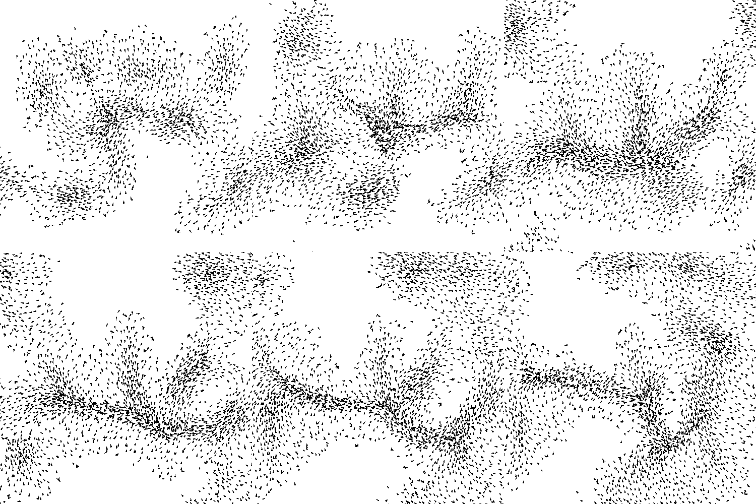
Note
Related to agent-based modelling.
Well-known type of agent-based system that realistically simulates the complex flocking behaviors of birds and fish using simple rules. Each "boid" is an autonomous agent that is only aware of its immediate neighbor boids, all following the same three rules:
- Separation (collision avoidance): steer to avoid crowding local flockmates
- Alignment (velocity matching): steer towards the average heading of local flockmates
- Note: remember that a vector is a combination of a speed and a direction (heading)!
- Cohesion (flock centering): steer to move towards the average position (center of mass) of local flockmates
And here is what those rules look like when applied to a set of agents (boids):
| Separation | Alignment | Cohesion |
|---|---|---|
 |
 |
 |
Additional rules can be implemented to simulate specific behaviors like obstacle avoidance, predator-prey interactions, bait balls, and more.
Articles:
- Flocks, Herds, and Schools: A Distributed Behavioral Model - original 1987 paper by Craig Reynolds
- Boids on Wikipedia
- Chapter 6. Autonomous Agents from Nature of Code
- Boids by Craig Reynolds
Code projects:
- Boids (source) by Marcio Puga (JavaScript, PixiJS)
Videos:
- Coding Challenge #124: Flocking Simulation by Daniel Shiffman (Github repo with source code for p5.js and Processing)

Technique for 3D solid modeling that allows for the creation of complex surfaces by using Boolean operators to combine simpler objects (usually primitives like cubes, spheres, cylinders, etc). Most CAD and 3D modeling applications (like Blender, Fusion, Rhino, and more) include CSG operations, sometimes even through parametric or procedural interfaces.
Operations:
| Name | Descriptionn | Illustration |
|---|---|---|
| Union | Merger of two objects into one |  |
| Difference | Subtraction of one object from another |  |
| Intersection | Portion common to both objects |  |
Articles:
- Constructive solid geometry on Wikipedia
Code projects:
- csg.js (JavaScript) by Evan Wallace
- CGAL 4.14- 3D Boolean Operations on Nef Polyhedra (C++)

Note
Related to verlet physics, particle systems, and physics engines.
Image credit: Isabel Zhang - Project 4: Cloth Simulator
Real-time simulation of cloth dynamics - how fabric bends, stretches, folds, and interacts with collisions and external forces like wind and gravity. Most cloth solvers model cloth as a mesh of particles connected by distance constraints (springs), typically using Verlet integration or Position Based Dynamics for stability and speed. The mesh deforms and settles as constraint-based solvers iteratively push connected particles toward their rest distances, while collisions are handled by detecting and pushing cloth away from obstacles.
Cloth simulation is essential for character animation, VFX, and any scenario requiring realistic fabric behavior without pre-baked animation. It scales from interactive real-time performance in games to high-quality offline rendering in film and animation.
Algorithm at a glance:
* indicates a potential simulation parameter
- Create a mesh of particles (one per vertex), each with mass*, position, and velocity.
- Connect neighboring particles with distance constraints (structural, shear, and optionally bend constraints*) representing fabric stiffness.
- Each frame, apply forces* (gravity, wind, damping) to all particles.
- Update particle positions using Verlet integration or similar.
- Repeatedly satisfy constraints: for each constraint, if the distance between two particles deviates from the rest length, nudge them toward the target distance.
- Optionally, check each constraint against a breaking threshold* (e.g., how much it can stretch before tearing); if exceeded, remove the constraint to simulate ripping or tearing.
- Detect collisions with rigid bodies and other geometry, and reposition particles to prevent penetration.
- Repeat until the cloth settles or the simulation ends.
Key terms:
- Structural constraint - distance constraint along the fabric's grid edges, prevents stretching.
- Shear constraint - diagonal distance constraint, prevents skewing and distortion.
- Bend constraint - constraint between particles separated by one edge, prevents unrealistic folding.
- Damping - friction-like force that slows particle motion over time, helps cloth settle faster.
- Self-collision - cloth colliding with itself; necessary for realistic folding and wrapping.
- Constraint breaking / tearing - removal of constraints when they exceed a strain threshold*, allowing cloth to rip and tear when stretched too far; can also be triggered by collision impact.
Articles:
- Cloth Modeling and Simulation: A Literature Survey in Springer's Computer Graphics and Geometric Modeling
- Simulation of Clothing with Folds and Wrinkles (PDF) by R. Bridson, S. Marino, and R. Fedkiw - foundational paper introducing a physically-correct bending model and wrinkle pre-shaping
- Robust Treatment of Collisions, Contact and Friction for Cloth Animation (PDF) by R. Bridson, R. Fedkiw, and J. Anderson - seminal paper on collision handling for cloth
- Fast Simulation of Cloth Tearing - techniques for efficiently simulating constraint breaking and mesh splitting during cloth tearing
- Simulation of Tearing Cloth with Frayed Edges - methods for realistic fraying and edge detail in torn cloth
- Breaking and Tearing - Houdini Vellum documentation on implementing constraint breaking and artistic control over tearing guides
Videos:
- Coding Challenge #63: Texturing and Cloth Simulation by Daniel Shiffman (The Coding Train) - combines toxiclibs Verlet physics with texture rendering for a waving flag
Notable tools:
- Obi Cloth (Unity asset) by Virtual Method - high-quality cloth simulation with character clothing, two-way rigidbody interaction, and aerodynamics
- Vellum (Houdini solver) by SideFX - unified cloth/hair/grain solver using Position Based Dynamics
Code projects:
- Cloth Simulation (p5.js) by Aryaman - interactive tearable cloth demo with wind and collisions

Computational methods for determining when two or more shapes are intersecting either statically (right now) or predictively (in the future). In technical terms, a posterior and a priori respectively. Detecting and reacting to collisions is extremely important in videos games and physical simulations, and takes quite a lot of brains and computational muscle to do effectively in real-time, especially in large-scale systems.
Building your own collision detection code is a fun and educational exercise, but is so complex and difficult to achieve in practice that it is generally a good idea to use an establisihed physics library or VFX/modelling application for performance. See the Physics engine and Tools sections for options.
Relevant topics:
- Broad phase - class of algorithms that detect pairs of potentially colliding shapes using fast but approximate methods, such as:
- Axis-aligned bounding box (AABB)
- Sort and sweep (a.k.a. sweep and prune)
- Bounding volume hierarchy (BVH)
- Narrow phase - class of algorithms that determine if two shapes are definately intersecting or not, and by how much.
- Separating axis theorem (SAT)
- Gilbert-Johnson-Keerthi (GJK) algorithm
- Expanding Polytope Algorithm (EPA)
Articles:
- Collision detection on Wikipedia
- Video Game Physics Tutorial - Part II: Collision Detection for Solid Objects by Nilson Souto
- Let's talk about broad phase by Stanislav Pidhorskyi
Books:
- Real-Time Collision Detection by Christer Ericson

Note
Related to convolution kernel.
In an image using a limited color palette, dithering can provide an illusion of a continuous gradient, or a field of color not in the palette. Using colors that are close to the target color, the technique applies a granular pattern of varying sizes and spacing of solid, single-color dots or lines. The human eye then interpolates between the colors at a larger scale.
Some techniques (like halftones) predate modern digital technologies because of their usefulness in traditional printmaking and engraving processes. There are even relevant techniques in the fields of painting and drawing; see stippling and pointillism! In digital imaging, modern palettes are usually comprehensive enough to reach a satisfactory visual fidelity for general purposes, but limits are still often reached in professional contexts.
Dithering is useful for realizing grayscale images with various digital fabrication equipment like laser cutters, pen plotters, CNC routers/mills, and more.
Types of dithering:
- Random
- Patterned
- Ordered
- Halftone ⭐
- Bayer matrix
- Blue noise matrix
- Error-diffusion
- Floyd-Steinberg ⭐
- Minimized average error
- Stucki
- Burkes
- Sierra
- Two-row Sierra
- Filter Lite
- Atkinson
- Gradient-based error-diffusion
Articles:
- Dither on Wikipedia
Code projects:
- Atkinson Dithering, Live in Processing by Windell Oskay of Evil Mad Scientist Laboratories
- Coding Challenge #90: Floyd-Steinberg Dithering by Daniel Shiffman (Github repo with source code for p5.js and Processing)
- Color Quantization and Dithering reference page for ImageMagick v6
- Digital Halftoning by C. A. Bouman
- #dithering-algorithms on Github
- Tramage (source) by Pierre Commenge - utility to dither small images and prepare machine knitting files. (p5.js and Processing)

Note
Related to fluid simulation.
Also known as a vector field, this technique involves assigning a unique vector to each point in a 2D or 3D space describing the direction and magnitude of varying forces. Flow fields are often used together with particle systems to model complex, dynamic movement caused by wind, fluid flow, electromagnetism, and more.
Vector fields are often populated using data generated with noise or image data. Curiously, flow fields have also been used in pathfinding.
Articles:
- Vector field on Wikipedia
- Flow Fields, Part I by Keith Peters
- Flow Fields, Part II by Keith Peters
Code projects:
- ofxVectorField (openFrameworks add-on) by Jeremy Rotzstain (mantissa)
Videos:
- Coding Challenge #24: Perlin Noise Flow Field by Daniel Shiffman (Github repo with source code for p5.js and Processing)

Note
Related to convolution kernels, Laplace equation, and Saffman–Taylor instability.
Simulates the highly complex and dynamic nature of flows in fluid volumes using computationally-efficient implementations of the Navier-Stokes equations. Can be thought of as a 2D or 3D flow field that is constantly changing based on the velocity, viscocity, and density of the fluid at each point in space and its surrounding area. This flow field is made visible through the use of digital "dyes" (usually particles) that get distributed, diffused, sheared, and blended through the system by the flow forces.
To appear realistic it is necessary for these simulations to have high fidelity, which introduces significant computational challenges, especially if one wants to run the simulation in real-time. Luckily, there are several great code packages available, and many VFX, CAD, and game development tools like Blender, Houdini, Unity and Unreal include robust fluid simulation functionality built in or available through plugins.
Fluid simulation has many practical and visual applications across a variety of disciplines. Its used in the analysis of aerodynamic properties of objects, vehicles, and buildings, in weather simulation and prediction, engine and combustion analysis, industrial systems design and analysis (plumbing, HVAC, public utilities, etc), visual effects for TV, movies, and games, and more.
Related terms:
- FLIP (FLuid Simulation Using Implicit Particles) method
- PIC (Particle in Cell) method
- Reynolds number (Re) - dimensionless quantity used to predict fluid flow patterns. Laminar (smooth) flow occurs at low Re, while turbulent flow occurs at high Re.
- Navier-Stokes equations on Wikipedia
- Lattice Boltzmann methods (LBM) on Wikipedia
- Rheology - branch of physics which deals with the deformation and flow of materials, both solids and liquids
Articles and papers:
- Fluid Simulation Using Implicit Particles (PDF) by Dan Englesson, Joakim Kilby, and Joel Ek
- Computational fluid dynamics (CFD) on Wikipedia
- Fluid Simulation for Dummies by Mike Ash
- Real-Time Fluid Dynamics for Games (PDF) by Jos Stam
- Chapter 38. Fast Fluid Dynamics Simulation on the GPU from GPU Gems book
Books:
- Fluid Simulation for Computer Graphics by Robert Bridson
Code projects:
- Lily Pad (Processing) by Dr. Gabriel David Weymouth
- MSAFluid by Memo Akten
- ofxMSAFluid (openFrameworks)
- p5-MSAFluid (Processing)
- OpenFOAM
- mantaflow
- Fluidity
Notable tools:
- FLIP Solver (Houdini)
- FLIP Fluids (Blender)
- Obi Fluids (Unity)
- Butterfly (Grasshopper for Rhino)
- RhinoCFD (Rhino)
- RealFlow (Standalone, or via plugins for 3ds Max, Maya, and Cinema4D)
Videos:
- Coding Challenge #132: Fluid Simulation by Daniel Shiffman (Github repo with source code for p5.js and Processing)
- Why Laminar Flow is AWESOME - Smarter Every Day 208 by Smarter Every Day

Note
Related to convolution kernel.
Image credit: Hrithik Patel - Kernels and Their Usage in Convolutional Neural Networks (CNN).
Applying convolution kernels to images for filtering and feature extraction. Each pixel's new value is computed as a weighted sum of its neighborhood, determined by the kernel matrix. This is one of the most practical and widely-used techniques in digital image processing.
Common image processing effects:
| Effect | Purpose | Kernel | Example |
|---|---|---|---|
| Edge detection (Sobel) | Detect boundaries between regions | |
 |
| Sharpen | Enhance edges and details | |
 |
| Box blur | Simple averaging blur | |
 |
| Gaussian blur | Smooth blur, weighted toward center | |
 |
| Unsharp mask | Enhance sharpness and clarity | |
 |
| Emboss | 3D relief effect | |
N/A |
Key implementation considerations:
- Boundary handling - what happens at image edges (zero-padding, reflection, wrapping, shrinking)
- Kernel normalization - dividing by kernel sum to preserve image brightness
- Separable kernels - 2D kernels that can be decomposed into two 1D operations for faster computation
- GPU acceleration - fragment shaders and compute shaders can apply kernels in parallel across many pixels
- Fixed-point math - integer-only math for embedded systems or performance-critical code
Articles:
- Kernel (image processing) on Wikipedia
- Image Kernels Explained Visually - interactive visualization
- Digital Image Processing on Wikipedia
- Kernels and Their Usage in Convolutional Neural Networks (CNN) by Hrithik Patel
Notable tools and libraries:
- OpenCV (C++, Python, JavaScript) - comprehensive image processing with custom kernels
- scikit-image (Python) - filters, morphology, edge detection
- PIL/Pillow (Python) -
ImageFiltermodule with predefined and custom kernels - GIMP - manual convolution filter tool (Filters > Generic > Convolution Matrix)
- Three.js postprocessing (JavaScript) - GPU-based kernel effects
- ImageMagick - command-line tool with
-morphologyand-convolveoperations

Note
Related to voronoi diagrams.
As explained by Jason Davies, Lloyd’s relaxation algorithm (named after Stuart P. Lloyd) generates a centroidal Voronoi tessellation, which is where the seed point for each Voronoi region is also its centroid.
The algorithm computes the Voronoi diagram for a set of points, moves each point towards the centroid of its Voronoi region, and repeats.
Important concepts:
- Convergence - every point that is being "relaxed" is moving towards the center point of a Voronoi cell, but due to computational limits in numerical precision it may not ever perfectly reach it. Therefore it is a good idea to use some sort of preset distance threshold value that causes points to stop moving once they are close enough to their target point.
Articles:
- Lloyd's algorithm on Wikipedia
- Voronoi relaxation (Lloyd's algorithm) in Processing by Alberto Giachino
Code projects:
- Javascript implementation of Steven Fortune's algorithm to compute Voronoi diagrams - Demo 5: Lloyd's relaxation by Raymond Hill (JavaScript) (source repo)
- Lloyd's Algorithm by Mike Bostock on Observable (JavaScript and D3.js)
- Lloyd's Relaxation by Luca Sbardella (JavaScript and D3.js)
- Lloyd's Relaxation by Jason Davies (JavaScript, see DOM for source code)

Method of generating contours for a 2D scalar field (a grid of individual numerical values), like turning elevation data into a banded topographical map. The scalar values get associated with vertices of the 2D grid, then lines are drawn across each cell in different ways based on the values of their four corner vertices.
There is only a finite number of lines possible, so they can be precomputed into a lookup table and referenced quickly later for faster performance. These lines can also be linearly interpolated to smoothly transition from cell to cell, resulting in very realistic blobby / fluid structures.
Key terms:
- Isoline - contour line tracing a single data level, or isovalue.
- Isoband - filled area between isolines.
Illustration of algorithm:

Articles:
- Marching squares on Wikipedia
- Metaballs and Marching Squares by Jamie Wong
Code projects:
- d3-contour - D3.js library
Videos:
- Marching Squares for procedural cave generation in Unity by Sebastian Lague

3D version of marching squares. Whereas marching squares uses lines and cells to trace the contours of a 2D scalar field, marching cubes uses polygons and voxels to trace the contours of a 3D scalar field, resulting in a mesh. Marching cubes can be thought of as a mesh conversion algorithm that produces meshes based on 3D scalar fields.
Originally developed by William Lorensen and Harvey Cline of General Electric in 1987 (see original paper in Articles section) for use in the medical imaging (MRI/CT) field, this algorithm has become widely used in many areas of computer graphics.
Dual marching cubes:
A variant called dual marching cubes (PDF) reverses the role of vertices and cells: instead of placing vertices on cube edges, it places vertices at voxel centers and connects them based on neighboring voxel values. This approach can reduce polygon count, better handle ambiguous cases at isovalue boundaries, and eliminate certain artifacts that appear in standard marching cubes. Dual marching cubes is particularly useful when a cleaner, more regular mesh is desired.
Algorithm [link]:
The algorithm proceeds through the scalar field, taking eight neighbor locations at a time (thus forming an imaginary cube), then determining the polygon(s) needed to represent the part of the isosurface that passes through this cube. The individual polygons are then fused into the desired surface.
- Choose a threshold (called an isovalue) to determine which level of values are considered inside or outside the mesh, thus setting where the mesh boundary is created.
- Pre-compute an array of all 256 (
2^8) possible polygon configurations within a cube, where each entry is a set of IDs associated with edges of the cube (see Figure B below).- Note that of these 256 configurations, only 15 are unique due to repetition and symmetry (see Figure A below).
- For each set of 8 scalar values (forming a cube), compute an 8-bit integer where each bit corresponds to a unique scalar value (corner of the cube).
- If the scalar value is higher than the isovalue (i.e. inside of mesh), set bit to 1
- If lower, set bit to 0
- Generate polygons for each set of scalar values by drawing lines between the edges referenced in the polygon lookup table from step 2.
- To do this, parse the 8 bits from step 3 into an integer, then use that integer as an index in the lookup table.
- For example
00101001=41. Therefore the list of edges to draw lines between can be found inlookupTable[41].
- Each vertex of the generated polygons is placed on the appropriate position along the cube's edge by linearly interpolating the two scalar values that are connected by that edge.
- Calculate normals - TODO: how?
- Perform boolean union with all polygon fragments to form a mesh
| (Figure A) diagram of 15 possible polygon configurations based on vertex bit values | (Figure B) diagram of edge and vertex numbering |
|---|---|
 |
 |
Key terms:
- Isosurface - surface that represents points of a constant value within a volume of space
Articles:
- Marching Cubes: A High-Resolution 3D Surface Construction Algorithm (PDF) - original paper by William Lorensen and Harvey Cline
- Marching cubes on Wikipedia
- Polygonising a scalar field by Paul Bourke
- Voxel to Mesh Conversion: Marching Cube Algorithm by Smile Sikand
Videos:
- Marching Cubes Animation by Algorithms Visualized

Note
Related to implicit surfaces, marching squares (2D) and marching cubes (3D).
Often confused with marching cubes, this is more of a mathematical concept that describes a way to define the values in 2D or 3D scalar fields based on distance to one or more points in space. They are a type of implicit surface that define blobby shapes as pure mathematical formulas rather than explicit polygons and vertices.
They can be visualized using the marching squares (2D) or marching cubes (3D) rendering algorithms. Can be used for naive fluid simulations by applying physics to the metaball center points as if they were particles. They can also be helpful in modelling soft bodies by adding elastic constraints between the center points.
A typical function chosen for metaballs is:
Where
Articles:
- Metaballs on Wikipedia
- Metaballs (also known as: Blobs) by Ryan Geiss
- Exploring Metaballs and Isosurfaces in 2D by Stephen Whitmore
Videos:
- Coding Challenge #28: Metaballs by Daniel Shiffman (Github repo with source code for p5.js and Processing)

Note
Related to convolution kernel.
In the context of computer graphics, refers to pseudo-random functions useful for creating natural-looking textures and patterns. Often used to procedurally generate organic surface textures (bark, waves, rocks, etc) and to organically distribute objects across surfaces (like grass or barnacles).
Useful for adding fine details and smooth asymmetry to otherwise pristine objects - use it in displacement maps for subtle natural features.
Also helpful for creating looping animations because reproducable results can be achieved when using the same function inputs. Just iterate through a series of cyclical values (perhaps even based on frame count) and you'll end up with smoothly transitioning noise that can be mixed in with geometry, colors, and transformations that continuously loop.
The noise() function in many creative coding frameworks usually makes use of Perlin noise.
- Curl noise - produces swirling, rotational motion patterns useful for simulating vortices, flowing fluids, and turbulent effects without the computational cost of a full physics simulation (see Curl-Noise for Procedural Fluid Flow (PDF) by Robert Bridson et al.)
- Gradient noise - created by interpolation of a lattice of pseudorandom gradients
- Perlin noise ⭐ - extremely influential type of gradient noise developed by Ken Perlin in 1983
- Simplex noise - method for constructing an n-dimensional noise function comparable to Perlin noise
- Simuation noise - function that creates a divergence-free field
- Value noise - created by interpolation of a lattice of pseudorandom values; differs from gradient noise
- Wavelet noise - alternative to Perlin noise which reduces problems of aliasing and detail loss
- Worley noise - noise function introduced by Steven Worley in 1996
Articles:
- Noise chapter in The Book of Shaders by Patricio Gonzalez Vivo & Jen Lowe
Videos:
- Coding Challenge #11: 3D Terrain Generation with Perlin Noise in Processing by Daniel Shiffman (Github repo with source code for p5.js and Processing)
- Coding Challenge #136.1: Polar Perlin Noise Loops by Daniel Shiffman (Github repo [2] with source code for p5.js and Processing)
Notable implementations:
- Curl noise
- Houdini - Curl Noise VOP
- Unreal Engine 5 - Procedural content documentation
- TouchDesigner - Curl Noise in Noise MAT
- GLSL - Curl noise shader implementations
- Bitangent noise - more computationally efficient alternative to curl noise for generating divergence-free vector fields (paper by Ivan DeWolf)
- Perlin noise
- Processing - built-in
noise()function - p5.js -
noise()function - Three.js / WebGL - SimplexNoise in examples; shader implementations
- Houdini - Noise VOP nodes (Perlin, Fractal, etc)
- TouchDesigner - Noise CHOP and Noise MAT operators
- vvvv - Noise nodes in vvvv.js and vvvv gamma
- Blender - Noise texture node in Shader Editor
- Processing - built-in
- Simplex noise
- GLSL - Simplex noise shader implementations (Ashima Arts)
- p5.js -
noise()uses Simplex noise - Houdini - Simplex Noise VOP
- TouchDesigner - available in Noise CHOP
- Blender - Noise texture with Simplex option
- Worley noise / Voronoi
- GLSL - Voronoi/Worley shader collections
- Houdini - Worley Noise VOP
- TouchDesigner - Voronoi/Worley operators
- Blender - Voronoi texture node in Shader Editor
- vvvv - Voronoi nodes in vvvv.js and vvvv gamma
Code projects:
- FastNoise2 (C++, multiple language bindings) - high-performance noise library with SIMD optimization
- libnoise (C++) - procedural noise library with multiple noise types
- Perlin Noise implementation collections (multiple languages)

Collection of independent objects (often points, shapes, images/sprites/textures, or meshes) called particles that are manipulated using dynamic forces and constraints to simulate a wide variety of natural phenomenon like fire, smoke/fog/clouds, fluids, bubbles, and so much more. Often combined with clever visual effects like transparency, blending, and light emission to create the appearance of a coherent but ever-changing entity.
Particle systems are most useful when they can handle large quantities of particles, which means that performance and smart memory management is very important. Like collision detection, building your own particle system can be fun and educational, but if you need to achieve something complex at a large scale and/or with high framerates then it's definitely a good idea to leverage dedicated libraries and tools. Many physics engines come with well-made particle systems out of necessity so be sure to consider them even if you don't need all the fun physics functionality.
Articles:
- Particle system on Wikipedia
- Intro to particle systems lesson on Khan Academy
- The physics of particle systems
- Chapter 4. Particle Systems from Nature of Code
Notable software:

Note
Related topics include collision detection and particle systems.
Simulates the movements and reactions of objects using real-world concepts like mass, velocity, constraints, and forces (like drag, gravity, and friction). Makes use of extremely optimized algorithms for collision detection, physics calculations, geometry management, and more.
Articles:
- Physics engine on Wikipedia
- Chapter 5. Physics Libraries from Daniel Shiffman's Nature of Code book
- How to Create a Custom 2D Physics Engine: The Basics and Impulse Resolution by Randy Gaul
Notable open-source libraries:
- Box2D (C++)
- Bullet (C++)
- ammo.js (direct JavaScript port using Emscripten)
- Matter.js (JavaScript)
- dyn4j (Java)
- cannon.js (JavaScript)
- p2.js (JavaScript)
- ReactPhysics3D (C++)
- Chrono (C++)
- Open Dynamics Engine (ODE) (C++)
Commercial libraries:
- PhysX by Nvidia. Integrated into both Unity and Unreal. Technically open-source now, but oriented more towards commercial/industry applications.
- Havok
If you're looking to do physical-based simulations, also take a look at game development and VFX environments like Unity, Unreal, and Houdini for their built-in physics engines.
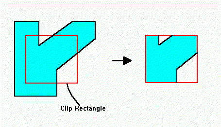
Effectively a Boolean intersection operation that "clips" (removes) parts of one polygon that are outside of another polygon. This can be useful when working with geospatial datasets and vector graphics (like SVGs), which in turn make this useful for plotter artists.
Algorithms:
Code projects:
- clipper-java by Tobias Mahlmann (Java)
- ofxClipper by Christopher Baker (openFrameworks / C++)
- polygon-clipping by Mike Fogel (JavaScript)

Rendering technique used to create photorealistic images of 3D scenes by tracing the path of individual light rays. Rather than simulate all light rays' journeys from every light source to the camera, only the light rays that actually reach the camera are simulated.
For each pixel of the screen, a ray is cast into the scene until it hits an object. Based on the scene's lighting and the material properties of the hit object, a color value is calculated for the corresponding screen pixel. Using the angle of the specific triangle that was hit along with material properties like surface roughness, refraction, diffusion, one can also determine what direction that light ray must have come from, tracing that path and incorporating it's color information into the pixel color calculation.
The number of "bounces" examined can increase the photorealism of the resulting image, at the cost of computational resources / time.
This process is extremely computationally expensive, so it has historically only been used in pre-rendered applications like movies, animations, and still images. However, recent advancements in graphics card technology (like NVIDIA's RTX series) are beginning to make this technique available in real-time applications.

Articles:
- Ray tracing (graphics) on Wikipedia
Code projects:

Note
Related to recursion.
Method of solving a problem where the solution depends on solutions to smaller instances of the same problem (as opposed to iteration). In programming terms, recursion is when a function calls itself during execution. Recursion is fundamentally connected to the concept of fractals.
Example: computing factorial
function factorialize(n) {
  if(n < 0) {
    return -1;
  } else if(n == 0) {
    return 1;
  } else {
    return n * factorialize(n - 1);
  }
}
Articles:
- Recursion on Wikipedia
- Recursion (computer science) on Wikipedia
- Droste effect on Wikipedia
Shaders are programs that are run on the GPU when processing a certain unit of rendering, usually vertices or pixels/fragments; they allow rendering programmers to manipulate their rendering output in any way they see fit.
While shaders, as the name implies, were originally conceived to allow different kinds of lighting/shading calculations, today they're used for a variety of things from lighting calculation through stylized rendering to 2D compositing or post-processing, and even complex geometry manipulations and particle effects.
Types of shaders:
Key concepts:
- FBO (framebuffer object)
- GPGPU (general-purpose computing on GPUs) - the concept of using the GPU to perform computation
- Ping pong - technique in which the output texture of one shader is fed to another shader as an input, sometimes cycling back and forth multiple times. The final texture gets sent to the display, then the shaders are swapped so that the most recent output becomes the input to the next iteration.
- Render to texture (RTT) - instead of rendering a scene to the screen, in this technique it is rendered to an "offscreen" texture that can be reused later.
- Shading language
- Textures
- Uniform - a type qualifier indicating a read-only variable passed to a shader from the CPU side of the program. These values will not change within a draw call, and are available to every shader that declares it.
- Varying - a type qualifier indicating a variable that can change within the vertex shader, then passed to the fragment shader as a read-only value.
Languages:
- Cg - shading language developed by Nvidia in close collaboration with Microsoft
- CUDA - parallel computing API that makes it easier to use GPGPU for complicated tasks
- GLSL (OpenGL Shading Language) - shading language used by OpenGL
- HLSL (High-Level Shading Language) - shading language used by DirectX
Articles:
- The Book of Shaders by Patricio Gonzalez Vivo and Jen Lowe
- Shaders by Learn OpenGL
- GLSL Shaders on MDN web docs
- Shaders (Processing) tutorial by Andres Colubi
- Introducing Shaders (openFrameworks) by Lucasz Karluk, Joshua Noble, Jordi Puig
- Shader modules (Vulkan)
Code tools:
Videos:
Note
Related to implicit surfaces.
A function that returns the distance between a point in space to a mathematically/algorithmically defined surface (called an implicit surface). This allows algorithms like raymarching and marching cubes to efficiently render complex 3D surfaces in 2D.
SDFs are increasingly commonly used in computer art, where defining an SDF that describes a large 3D scene entirely in a single pixel shader allows the code to be ran entirely on the GPU.
Articles:
- Signed distance function on Wikipedia
- Distance functions (GLSL)
- Ray Marching and Signed Distance Functions by Jamie Wong
Notable open-source libraries:
- hg_sdf (GLSL)
Videos:

Note
Related to mass-spring systems, cloth simulation, Verlet physics, and physics engines.
Image credit: CoppeliaSim docs - Physics engine differences
Soft-body physics is the applied, real-time counterpart to mass-spring systems: simulating volumetric objects - rubber, flesh, jelly, foam, organs - that deform under force and recover their shape rather than staying rigid. Unlike cloth simulation, which models thin 2D sheets, soft-body solvers operate on 3D volumes (tetrahedral meshes, voxel grids, or particle clouds) and must resist compression as well as stretching, giving deformable objects a sense of internal volume and squishiness.
Several families of techniques compete for this problem, each trading accuracy for speed differently:
- Mass-spring - the volumetric extension of mass-spring systems: tetrahedral or lattice structures of point masses connected by springs. Fast and simple, but prone to visible artifacts (bulging, asymmetric stretching) since spring networks don't perfectly capture rotational/volumetric behavior.
- Finite Element Method (FEM) - discretizes the body into tetrahedral elements and solves continuum-mechanics stress/strain equations directly, giving physically accurate results at higher computational cost. Common in engineering, biomechanics, and high-end VFX.
- Shape matching - a meshless technique that computes a "goal" rigid/deformed shape for a cluster of particles each frame and pulls particles toward it; cheap, stable, and popular in games.
- Position Based Dynamics (PBD) / XPBD - treats constraints (distance, volume, bending) as positional corrections solved iteratively rather than forces, which is unconditionally stable and easy to combine with cloth, rigid bodies, and fluids in one solver. XPBD adds proper stiffness independent of iteration count and time step.
Key terms:
- Tetrahedral mesh - the volumetric equivalent of a triangle mesh; most FEM and volumetric mass-spring solvers discretize a soft body into tetrahedra.
- Volume constraint - a constraint that resists compression/expansion of a tetrahedron or cell, preventing unrealistic "deflating" under stress.
- Stress and strain - core FEM quantities describing internal forces and deformation, related through a material's stiffness (its constitutive model).
- Shape matching - fitting a rigid or affine transform to a rest-shape point cluster each frame, then pulling particles toward the transformed goal positions.
- Corotational formulation - a technique used in FEM/mass-spring elasticity models to separate rotation from strain, avoiding ghost forces when elements rotate.
Articles:
- Soft-body dynamics on Wikipedia
- Meshless Deformations Based on Shape Matching (PDF) by Müller, Heidelberger, Teschner, and Gross - foundational shape-matching paper
- Position Based Dynamics (PDF) by Müller, Heidelberger, Hennix, and Ratcliff
- XPBD: Position-Based Simulation of Compliant Constrained Dynamics (PDF) by Macklin, Müller, and Chentanez
- FEM Simulation of 3D Deformable Solids: A Practitioner's Guide - SIGGRAPH course by Sifakis and Barbič covering FEM soft-body simulation from first principles
Videos:
- Coding Challenge 177: Soft Body Physics by Daniel Shiffman (Coding Train)
- Ten Minute Physics by Matthias Müller - short tutorials covering shape matching, PBD, XPBD, and soft-body simulation from scratch
- 10 - Simple and unbreakable simulation of soft bodies by Ten Minute Physics
Notable tools and libraries:
- PositionBasedDynamics (C++) by Jan Bender - open-source PBD/XPBD library covering cloth, soft bodies, fluids, and rigid bodies
- SOFA - open-source framework for real-time multi-physics simulation, widely used in biomedical soft-tissue and soft-robotics research
- PhysX 5 by NVIDIA - GPU-accelerated FEM-based soft body simulation, open-sourced from the former NVIDIA Flex library
- Unity
- Obi Softbody by Virtual Method - particle-based soft body simulation
- Unreal
- TouchDesigner
- Flex - GPU particle solver (Nvidia Flex) for particle-based soft materials and fluids
- Processing
- toxiclibs - Verlet-based particle/spring physics library commonly used for soft-body and cloth-like simulations
- p5.js
- p5-matter - wraps Matter.js's soft-body composite meshes
- toxiclibs.js - JavaScript port of toxiclibs
- Three.js
- Ammo.js soft body volume demo (first-party) - official three.js example using the Bullet-based Ammo.js soft body solver
- React Three Fiber
- use-ammojs - Ammo.js/Bullet physics hooks with soft body
- Houdini
- Vellum - unified PBD solver for cloth, hair, grains, and soft bodies
- Blender
- Soft Body- built-in mass-spring-based soft body physics
Code projects:
- Ten Minute Physics - Soft Bodies by Matthias Müller - self-contained XPBD soft-body demo in vanilla JavaScript
- ammo.js Soft Body Volume demo - Bullet physics soft-body simulation ported to the web via three.js
- Soft Body Character by The Coding Train - p5.js soft-body character built with toxiclibs.js springs and particles

Data structure (most commonly a binary tree) that enables fast and efficient storage, manipulation, and querying of large amounts of spatial data (points in space). Commonly used by particle systems.
Common types:
- Quadtree - each node has exactly four children
- Octree - each node has exactly eight children
- k-d tree
- R-tree
Related topics:
- k-nearest neighbhor (knn) search
- Spatial database on Wikipedia
- Binary space partitioning on Wikipedia
Articles:
- Spatial index section on Wikipedia article for Spatial database
Videos:

Vectors (specifically Euclidean or geometric vectors) are simple data structures that store spatial information representing discrete points, displacement, or forces. Understanding how to work with vectors is one of the most critical skills to learn when working with physically-based simulations and digital morphogenesis.
Vectors can be manipulated using familiar algebraic operations like addition, subtraction, multiplication, and division, which makes them extremely useful when simulating physically-based systems with objects (or agents) in motion. We can have one vector that represents a point in space and another that represents a force (like gravity or wind), then apply that force to the point by adding the two vectors together.
The term "vector" has slightly different meanings and uses in mathematics, physics, machine learning, biology, and more. In the context of digital morphogenesis, you'll most often encounter vectors as they are used in physics, representing discrete physical properties like position, displacement, velocity, direction, and more.
Properties:
-
Magnitude / length (
$|\mathbf{v}|$ ) = the "size" of a vector obtained by taking the square root of the sum of the square of each of the vector's components (an abstraction of the Pythagorean Formula). Mathematically,$|\mathbf{v}| = \sqrt{v_x^2 + v_y^2 + v_z^2 + \ldots}$ . - Heading / direction / angle = the direction in which a vector is pointing. Applicable when using vectors to represent forces, but not so much when representing discrete points in space.
Key concepts:
- Unit vector = any vector with a magnitude (length) of exactly 1.
- Normalization = operation whereby a vector is divided by its own magnitude, resulting in a unit vector with the same heading (direction) as the original vector.
Algebraic operations:
| Operation | Using two vectors | Using a vector and a scalar |
|---|---|---|
| Addition | ||
| Subtraction | ||
| Multiplication | ||
| Division | ||
| Dot product |
(produces a single number) |
Not applicable. |
| Cross product |
Where: |
Not applicable. |
Articles:
- Euclidean vector on Wikipedia
- Chapter 1. Vectors in The Nature of Code by Daniel Shiffman
- Vectors from Math is Fun
Videos:
- What is a Vector? - Nature of Code lesson #1.1 by Daniel Shiffman
- Getting Started with Vector Math - Nature of Code lesson #1.2 by Daniel Shiffman
- A Random Vector - Nature of Code lesson #1.3 by Daniel Shiffman
- Unit: Vectors series from Khan Academy
Notable implementations:
- PVector in Processing (JavaDoc reference and source code)
- p5.Vector in p5.js
- Vector2, Vector3, and Vector4 in Three.js
- ofVec2f and ofVec3f in openFrameworks
- Vector data types in GLSL
- Vector Type in HLSL
- Vector2, Vector3, Vector4 in Unity

Note
Related or similar to spatial indices and fluid simulations
Image credit: Said Al Attrach - VDB: A Deep Dive
Grid-based data structure designed for storing and manipulating sparse 3D volumetric data - grids of voxels (3D pixels). Unlike a naive 3D array where every voxel consumes memory regardless of content, VDBs use a B-tree-like hierarchical structure that only stores voxels containing meaningful data, making them extremely memory-efficient for large, sparse volumes. Named for their characteristics (Volumetric, Dynamic, and B-tree-like), they approximate an "infinite" index space with fast O(1) random access, cache-coherent traversal, and support for dynamic topology changes.
VDBs are the industry standard in VFX and animation for representing volumetric data like smoke, fire, liquids, and distance fields. OpenVDB, an Academy Award-winning open-source library originally developed by DreamWorks Animation, has become the de facto standard format for volumetric data interchange in professional VFX pipelines.
How they work at a glance:
The VDB hierarchy typically has four levels: a root node (hash table), intermediate nodes, and leaf nodes (storing fixed blocks of voxels, usually 8×8×8). When accessing or inserting data, the tree is traversed from root to leaf, skipping branches that contain no data. This structure avoids allocating memory for empty space while maintaining fast random access patterns typical of dense grids.
Articles:
- VDB: High-Resolution Sparse Volumes with Dynamic Topology (PDF) by Ken Museth - the foundational 2013 ACM Transactions on Graphics paper introducing VDB at DreamWorks Animation
Notable tools and libraries:
- ⭐ OpenVDB (C++, Python bindings) by Academy Software Foundation
- GitHub repo - open-source, cross-platform library maintained by the VFX industry
- Official docs - API reference and guides
- Includes tools for data I/O, visualization (vdb_view), filtering, and mesh generation
- Blender
- Volume objects - native VDB/OpenVDB volume support
- Import VDB Geometry Node
- EmberGen - real-time volumetric fluid simulator using VDB-compatible formats for export
- Houdini
- OpenVDB volumes - native VDB support
- Three.js
- mjurczyk/openvdb - adds
.vdbformat support with a VDBLoader as well as aFogVolumeclass for working with the data
- mjurczyk/openvdb - adds
Code projects:
- fluid-engine-OpenVDB (C++) - fluid simulation engine adapting algorithms from fluid-engine-dev to leverage OpenVDB's sparse structure for memory-efficient 3D grid-based physics
- Liquid3D (C++) - IISPH (Implicit Incompressible SPH) fluid simulation that uses OpenVDB to mesh fluid particles for Blender import
- OpenVDB_Visualizer (C++) - volume rendering application using OpenGL and Qt5 to visualize and explore VDB files

Note
Related to Tiling / tessellation.
Method of procedurally generating textures and tilemaps that are similar to a single source image using ideas from quantum mechanics. Originally developed by Maxim Gumin, WFC learns local patterns and constraints from a source image, then iteratively generates new content by "collapsing" possibilities while respecting learned rules. The name references quantum superposition (many possible states simultaneously) and measurement (collapsing to a single outcome).
The algorithm works in two main steps: first, extract patterns by scanning the source image and recording which local arrangements of pixels (or tiles) occur; second, generate output by starting with all possibilities everywhere, then repeatedly choosing a location with minimum entropy (fewest valid options) and randomly collapsing it to one valid choice, then propagating constraints to neighbors to ensure the result remains compatible.
The key insight is that local compatibility - enforcing that neighboring regions respect learned patterns - naturally produces globally coherent, recognizable results even though the algorithm makes only local decisions. This approach produces remarkably human-like outputs and has become popular for game level design, texture synthesis, and procedural content generation.
Algorithm outline:
* indicates a potential simulation parameter
- Scan the source image to extract all
$N \times N$ * local patterns (e.g., all 3×3 neighborhoods of pixels or tiles). - Initialize the output grid with all patterns marked as possible at every location.
- In each iteration:
- Find the location with minimum entropy (fewest valid patterns remaining).
- If no location remains, generation is complete.
- If a location has zero valid patterns (contradiction), backtrack or restart.
- Randomly select one valid pattern from that location and collapse it (remove all other patterns).
- Propagate constraints: for each neighbor, remove any patterns that would be incompatible with the collapsed pattern (based on learned adjacencies).
- Repeat until the entire grid is determined.
Key terms:
- Pattern extraction - scanning the source image to find all valid local neighborhoods.
- Entropy - in this context, the number of valid choices remaining at a location; minimum entropy heuristic prioritizes constrained areas.
- Wave - the superposition of all possible patterns at each location before collapse.
- Collapse - randomly choosing one pattern and removing all alternatives.
- Constraint propagation - updating neighbors to eliminate patterns incompatible with a collapsed choice; ensures global coherence.
- Contradiction / backtracking - if all patterns are eliminated at some location, the algorithm has failed and must restart or undo recent decisions.
- Tile-based vs. pixel-based - the algorithm works on discrete units (tiles for maps, pixels for images) and can be adapted to 2D or 3D.
Articles:
- Original WaveFunctionCollapse Github repo by Maxim Gumin (mxgmn)
- Generating Worlds With Wave Function Collapse by Joseph Parker
- Doodle Insights #19: Logic Data Generation (feat. WFC made easy) by Rémy Devaux (TRASEVOL_DOG)
Code projects:
Videos:
- WaveFunctionCollapse Supercharged with PDG for Level Generation talk by Paul Ambrosiussen at HOUDINI HIVE GAMEDEV

Note
Related to Delaunay triangulation and Voronoi diagrams, dithering, and Lloyd's relaxation.
Image credit: Windell Oskay (Evil Mad Scientist Laboratories) - StippleGen: Weighted Voronoi stippling and TSP paths in Processing.
Weighted variant of Lloyd's relaxation that uses the darkness (or density) of an underlying image to bias where points settle, producing a stippled illustration made of dots whose size and/or spacing follows the image's tone - more and/or larger dots in darker regions, fewer/smaller dots in lighter ones. Because points are still spread evenly within their local Voronoi region even as they respect image density, the result reads as a convincingly hand-drawn stipple illustration rather than a mechanical dither pattern.
Frequently paired with TSP path-finding to connect the stippled points into a single continuous line, making it a popular technique for pen plotter art.
Algorithm at a glance:
- Scatter an initial set of points across the image, with more points landing in darker regions (e.g. via rejection sampling against pixel brightness).
- Compute the Voronoi diagram for the current points.
- For each Voronoi cell, compute its centroid using the underlying image as a density function - darker pixels pull the centroid more strongly - rather than treating every pixel in the cell equally, as in standard Lloyd's relaxation.
- Move each point to its cell's weighted centroid.
- Repeat for some number of iterations*, or until points stop moving significantly.
- Render each final point as a dot, optionally sized or oriented based on local density.
* indicates a potential simulation parameter
Key terms:
- Density function - the underlying image data used to weight where points are pulled during relaxation; typically derived from pixel brightness/darkness.
- Weighted centroid - center of mass of a Voronoi cell computed using the density function, as opposed to the plain geometric centroid used in standard Lloyd's relaxation.
Articles:
- Weighted Voronoi Stippling (PDF) by Adrian Secord. The original 2002 paper.
- Weighted Voronoi Stippling by Nicolas Rougier - a peer-reviewed reproduction of Secord's algorithm published in ReScience (2017).
- Creating Traveling Salesman Art With Weighted Voronoi Stippling by Jack Morris
Videos:
- Coding Challenge #181: Weighted Voronoi Stippling by Daniel Shiffman (p5.js and d3.js)
Notable software:
- StippleGen by Evil Mad Scientist Laboratories - Processing-based tool that generates weighted Voronoi stipple drawings, including TSP path art.
- Voronoi Stippling Art Generator by Joe Shenouda - browser-based tool for turning any photo into a stipple drawing
Creative projects:
Code projects:
- Swingline by Matt Keeter - C implementation that runs up to 10-20x faster than StippleGen (Github repo)
- Voronoi Stippling by Mike Bostock on Observable (JavaScript and D3.js)
- weighted-voronoi-stippling by Amaury Sanchez (JavaScript) - straightforward reference implementation of Secord's algorithm
- weighted-voronoi-stippling by Juha Tompuri (Python) - high-performance, Numba-accelerated implementation that exports PNG and TSP tour files
- Stippling and TSP art by Simon Barthelmé - tutorial with runnable code using the
imagerR package
- Animal Architecture by Ingo Amdt and Jurgen Tautz
- Art Forms from the Ocean: The Radiolarian Prints of Ernst Haeckel by Olaf Breidbach
- Art Forms in Nature by Ernst Haeckel
- Fractal Concepts in Surface Growth by Albert-László Barabási
- Fractal Growth Phenomena by Tamas Vicsek
- Nature's Patterns: A Tapestry in Three Parts by Philip Ball
- On Growth and Form by D'Arcy Wentworth Thompson
- The Algorithmic Beauty of Sea Shells by Hans Meinhardt
- Nervous System - Eyeo Festival 2011
- Algorithmic Design with Houdini by Junichiro Horikawa at SIGGRAPH Asia 2018
TODO: Add link


 Entagma's Patreon series
| Application | Description | Cost |
|---|---|---|
| Houdini | Industry-level procedural VFX application with graphical node-based workflow. Excellent for creating high-quality renderings and animations based on generative algorithms. Allows for scripting with Python and VEX (proprietary language). |
|
| Rhino | NURBS-based CAD program popular with architects and industrial designers. Strong ecosystem of advanced computational design plugins built by highly skilled community. Less focus on rendering, animation, and interactivity; more for form-finding with fabrication in mind. Allows for scripting with Python, RhinoScript, and more.List of useful Rhino plugins
|
|
| Unity |
Full-featured game engine with tools for interactivity, physics, lighting, level/character design, and more. Allows for scripting with C#. Direct competitor of Unreal, with a reputation for being more focused on "user friendliness" and less on hyper-realism, though the gap is shrinking rapidly. Notable features
|
|
| Unreal | Full-featured game engine with very similar feature set to Unity (it's direct competitor). Has reputation for being more focused on hyper-realism, and thus is used more by high-end games studios. [?] |
Free with royalty on commercial products |
| Structure Synth | Application for generating surprising and complex fractal 3D structures using a design grammar. | Free |
| TouchDesigner | Visual node-based environment for real-time interactive multimedia content useful for performances, installations, and fixed media works. Has roots in Houdini 4 and is considered a spin-off optimized for real-time performance work (hence the company name, Derivative). |
|
| Cinema 4D | Four versions ranging from $995-$3695 |
- Shaders
- C++
- Go
- JavaScript
- Java
- Rust
- Kotlin
