Image processing is the technique of analyzing and manipulating digital images using computational methods to extract information, enhance quality, or perform specific tasks. With powerful libraries such as OpenCV, Python provides an efficient environment for implementing a wide range of image processing operations.
- Supports operations such as image enhancement, feature extraction, object detection, and segmentation.
- Provides efficient tools for processing both images and videos in real-world applications.
Image Processing Using OpenCV
OpenCV is an open-source computer vision library that supports multiple programming languages, including Python, C++, and Java. It provides tools for image processing, feature extraction, and object detection, making it widely used in real-time, research, and industrial applications.
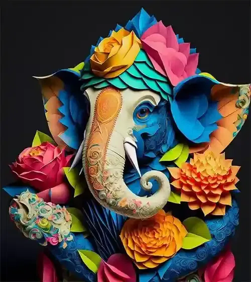
Input Image :
1. Image Resizing
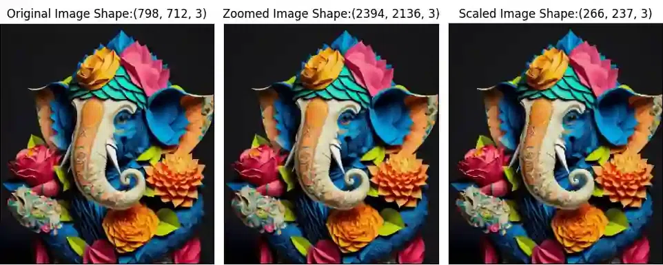
Image resizing is the process of changing the dimensions of an image by either enlarging or reducing its size while preserving the visual content. It is commonly used to adapt images for display, storage, or further image processing tasks.
cv2.resize()is used to resize an image to specified dimensions.cv2.INTER_CUBICis preferred for image enlargement, whilecv2.INTER_AREAis suitable for downscaling images.
import cv2
import numpy as np
import matplotlib.pyplot as plt

image = cv2.imread('Ganeshji.webp')
image_rgb = cv2.cvtColor(image, cv2.COLOR_BGR2RGB)
scale_factor_1 = 3.0
scale_factor_2 = 1/3.0
height, width = image_rgb.shape[:2]
new_height = int(height * scale_factor_1)
new_width = int(width * scale_factor_1)

zoomed_image = cv2.resize(src =image_rgb,
                          dsize=(new_width, new_height),
                          interpolation=cv2.INTER_CUBIC)

new_height1 = int(height * scale_factor_2)
new_width1 = int(width * scale_factor_2)
scaled_image = cv2.resize(src= image_rgb,
                          dsize =(new_width1, new_height1),
                          interpolation=cv2.INTER_AREA)

fig, axs = plt.subplots(1, 3, figsize=(10, 4))
axs[0].imshow(image_rgb)
axs[0].set_title('Original Image Shape:'+str(image_rgb.shape))
axs[1].imshow(zoomed_image)
axs[1].set_title('Zoomed Image Shape:'+str(zoomed_image.shape))
axs[2].imshow(scaled_image)
axs[2].set_title('Scaled Image Shape:'+str(scaled_image.shape))

for ax in axs:
    ax.set_xticks([])
    ax.set_yticks([])

plt.tight_layout()
plt.show()
Output:
2. Image Rotation
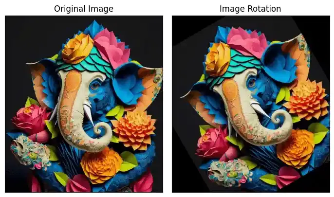
Image rotation is the process of rotating an image by a specified angle in clockwise or anticlockwise direction. It is commonly used for image augmentation and alignment.
cv2.getRotationMatrix2D()creates the rotation matrix using center point, angle, and scale.cv2.warpAffine()applies the rotation transformation to the image.- Positive angles rotate clockwise, while negative angles rotate anticlockwise.
import cv2
import matplotlib.pyplot as plt
img = cv2.imread('Ganeshji.webp')
image_rgb = cv2.cvtColor(img, cv2.COLOR_BGR2RGB)
center = (image_rgb.shape[1] // 2, image_rgb.shape[0] // 2)
angle = 30
scale = 1
rotation_matrix = cv2.getRotationMatrix2D(center, angle, scale)
rotated_image = cv2.warpAffine(image_rgb, rotation_matrix, (img.shape[1], img.shape[0]))

fig, axs = plt.subplots(1, 2, figsize=(7, 4))
axs[0].imshow(image_rgb)
axs[0].set_title('Original Image')
axs[1].imshow(rotated_image)
axs[1].set_title('Image Rotation')
for ax in axs:
    ax.set_xticks([])
    ax.set_yticks([])

plt.tight_layout()
plt.show()
Output:
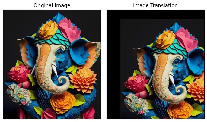
3. Image Translation
Image Translation is the process of moving an image from one position to another within a specified frame of reference. This shift can occur along the x-axis (horizontal movement) and y-axis (vertical movement) without altering the content or orientation of the image.
cv2.warpAffine()shifts the image based on translation values.tx, tydefine the movement along the x and y axes.
import cv2
import matplotlib.pyplot as plt
import numpy as np

img = cv2.imread('Ganeshji.webp')
image_rgb = cv2.cvtColor(img, cv2.COLOR_BGR2RGB)
width, height = image_rgb.shape[1], image_rgb.shape[0]

tx, ty = 100, 70
translation_matrix = np.array([[1, 0, tx], [0, 1, ty]], dtype=np.float32)
translated_image = cv2.warpAffine(image_rgb, translation_matrix, (width, height))

fig, axs = plt.subplots(1, 2, figsize=(7, 4))
axs[0].imshow(image_rgb), axs[0].set_title('Original Image')
axs[1].imshow(translated_image), axs[1].set_title('Image Translation')

for ax in axs:
    ax.set_xticks([]), ax.set_yticks([])

plt.tight_layout()
plt.show()
Output:
4. Image Shearing
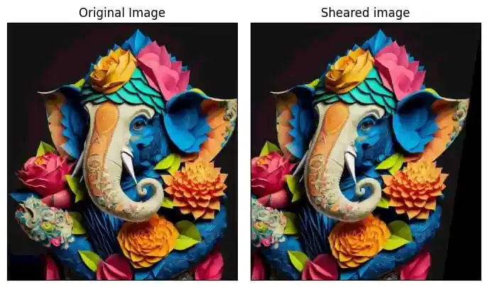
Image Shearing is a geometric transformation that distorts or skews an image along one or both axes. This operation slants the image creating a shear effect without changing its area or shape. Shearing can be applied to make the image appear as if it’s being stretched or compressed in a particular direction. Here:
shear_x, shear_ycontrol the degree of skewing.cv2.warpAffine()applies the transformation.
import cv2
import numpy as np
import matplotlib.pyplot as plt

image = cv2.imread('Ganeshji.webp')
image_rgb = cv2.cvtColor(image, cv2.COLOR_BGR2RGB)
width, height = image_rgb.shape[1], image_rgb.shape[0]

shearX, shearY = -0.15, 0
transformation_matrix = np.array([[1, shearX, 0], [0, 1, shearY]], dtype=np.float32)
sheared_image = cv2.warpAffine(image_rgb, transformation_matrix, (width, height))

fig, axs = plt.subplots(1, 2, figsize=(7, 4))
axs[0].imshow(image_rgb), axs[0].set_title('Original Image')
axs[1].imshow(sheared_image), axs[1].set_title('Sheared Image')

for ax in axs:
    ax.set_xticks([]), ax.set_yticks([])

plt.tight_layout()
plt.show()
Output:
5. Image Normalization
Image Normalization scales pixel values to a specific range to enhance image processing tasks. Here:
cv2.normalize() normalizes pixel values.cv2.NORM_MINMAX scales values between 0 and 1.cv2.merge() combines separately normalized RGB channels.
import cv2
import numpy as np
import matplotlib.pyplot as plt

image = cv2.imread('Ganeshji.webp')
image_rgb = cv2.cvtColor(image, cv2.COLOR_BGR2RGB)
b, g, r = cv2.split(image_rgb)

b_normalized = cv2.normalize(b.astype('float'), None, 0, 1, cv2.NORM_MINMAX)
g_normalized = cv2.normalize(g.astype('float'), None, 0, 1, cv2.NORM_MINMAX)
r_normalized = cv2.normalize(r.astype('float'), None, 0, 1, cv2.NORM_MINMAX)

normalized_image = cv2.merge((b_normalized, g_normalized, r_normalized))
print(normalized_image[:, :, 0])

plt.imshow(normalized_image)
plt.xticks([]),
plt.yticks([]),
plt.title('Normalized Image')
plt.show()
Output:
[[0.0745098 0.0745098 0.0745098 ... 0.07843137 0.07843137 0.07843137]
[0.0745098 0.0745098 0.0745098 ... 0.07843137 0.07843137 0.07843137]
[0.0745098 0.0745098 0.0745098 ... 0.07843137 0.07843137 0.07843137]
...
[0.00392157 0.00392157 0.00392157 ... 0.0745098 0.0745098 0.0745098 ]
[0.00392157 0.00392157 0.00392157 ... 0.0745098 0.0745098 0.0745098 ]
[0.00392157 0.00392157 0.00392157 ... 0.0745098 0.0745098 0.0745098 ]]
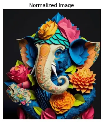
- A pixel value of 0.0745098 means the original pixel value was around 19 on the 0-255 scale (since 0.0745098 * 255 ≈ 19). It's a low intensity but not completely dark.
- A pixel value of 0.00392157 means the original pixel value was around 1 on the 0-255 scale (0.00392157 * 255 ≈ 1) which is very close to black or no color.
6. Edge detection of Image
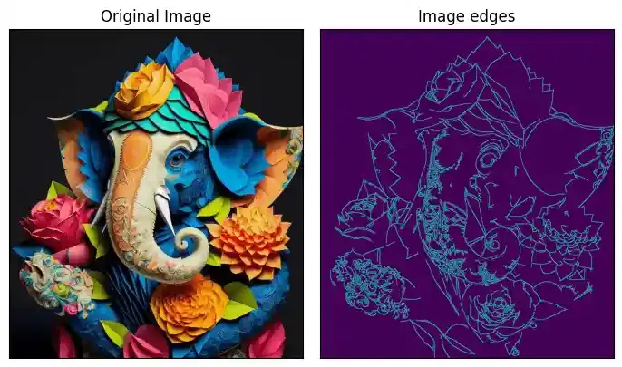
Edge detection is used to find sharp edges withing image to find different objects and boundaries within a image. Canny Edge Detection is a popular edge detection method.
cv2.GaussianBlur() removes noise through Gaussian smoothing.cv2.Sobel() computes the gradient of the image.cv2.Canny() applies non-maximum suppression and hysteresis thresholding to detect edges.
import cv2
import numpy as np
import matplotlib.pyplot as plt

img = cv2.imread('Ganeshji.webp')
image_rgb = cv2.cvtColor(img, cv2.COLOR_BGR2RGB)
edges = cv2.Canny(image_rgb, 100, 700)

fig, axs = plt.subplots(1, 2, figsize=(7, 4))
axs[0].imshow(image_rgb), axs[0].set_title('Original Image')
axs[1].imshow(edges), axs[1].set_title('Image Edges')

for ax in axs:
    ax.set_xticks([]), ax.set_yticks([])

plt.tight_layout()
plt.show()
Output:
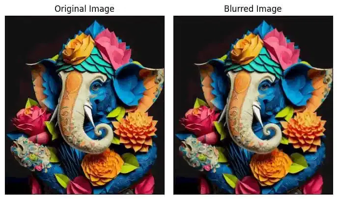
7. Image Blurring
Image Blurring reduces image detail by averaging pixel values.
cv2.GaussianBlur() smooths using a Gaussian kernel.cv2.medianBlur() replaces pixels with the median value in a neighborhood..cv2.bilateralFilter() preserves edges while blurring.
import cv2
import numpy as np
import matplotlib.pyplot as plt

image = cv2.imread('Ganeshji.webp')
image_rgb = cv2.cvtColor(image, cv2.COLOR_BGR2RGB)
blurred = cv2.GaussianBlur(image, (3, 3), 0)
blurred_rgb = cv2.cvtColor(blurred, cv2.COLOR_BGR2RGB)

fig, axs = plt.subplots(1, 2, figsize=(7, 4))
axs[0].imshow(image_rgb), axs[0].set_title('Original Image')
axs[1].imshow(blurred_rgb), axs[1].set_title('Blurred Image')

for ax in axs:
    ax.set_xticks([]), ax.set_yticks([])

plt.tight_layout()
plt.show()
Output:
8. Morphological Image Processing
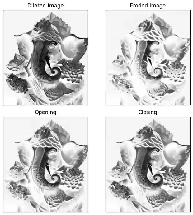
Morphological image processing refers to techniques that modify the shape and structure of objects in an image using a defined kernel. It is commonly used for noise removal, shape refinement, and feature enhancement.
cv2.dilate()expands object boundaries in an image.cv2.erode()shrinks object boundaries and removes small details.cv2.morphologyEx()performs advanced operations like opening (noise removal) and closing (hole filling).
import cv2
import numpy as np
import matplotlib.pyplot as plt

image = cv2.imread('Ganeshji.webp')
image_gray = cv2.cvtColor(image, cv2.COLOR_BGR2GRAY)
kernel = np.ones((3, 3), np.uint8)

dilated = cv2.dilate(image_gray, kernel, iterations=2)
eroded = cv2.erode(image_gray, kernel, iterations=2)
opening = cv2.morphologyEx(image_gray, cv2.MORPH_OPEN, kernel)
closing = cv2.morphologyEx(image_gray, cv2.MORPH_CLOSE, kernel)

fig, axs = plt.subplots(2, 2, figsize=(7, 7))
axs[0, 0].imshow(dilated, cmap='Greys'), axs[0, 0].set_title('Dilated Image')
axs[0, 1].imshow(eroded, cmap='Greys'), axs[0, 1].set_title('Eroded Image')
axs[1, 0].imshow(opening, cmap='Greys'), axs[1, 0].set_title('Opening')
axs[1, 1].imshow(closing, cmap='Greys'), axs[1, 1].set_title('Closing')

for ax in axs.flatten():
    ax.set_xticks([]), ax.set_yticks([])

plt.tight_layout()
plt.show()
Output: