Wolfram Function Repository
Instant-use add-on functions for the Wolfram Language
Function Repository Resource:
Find the best fitting line with respect to orthogonal distance
ResourceFunction["OrthogonalLineFit"][data] finds the best fitting orthogonal distance regression line to data. |
Parameters for a 2D line:
| In[1]:= | ![BlockRandom[SeedRandom[42, Method -> "ExtendedCA"];
{p0, v0} = {RandomReal[{-2, 2}, 2], Normalize[RandomVariate[NormalDistribution[], 2]]}]](https://www.wolframcloud.com/obj/resourcesystem/images/115/115b0475-c4a7-41e2-aca2-d63d90fe1a4c/551d91cb8b57166a.png) |
| Out[1]= |  |
Generate some points near the line:
| In[2]:= | ![BlockRandom[SeedRandom[42, Method -> "ExtendedCA"];
pts = Table[
p0 + t v0 + RandomVariate[NormalDistribution[0, 1/15], 2], {t, RandomReal[1, 25]}]]](https://www.wolframcloud.com/obj/resourcesystem/images/115/115b0475-c4a7-41e2-aca2-d63d90fe1a4c/2674c7ff16f8a267.png) |
| Out[2]= |  |
Find the orthogonal distance regression line:
| In[3]:= | ![ofit = ResourceFunction["OrthogonalLineFit"][pts]](https://www.wolframcloud.com/obj/resourcesystem/images/115/115b0475-c4a7-41e2-aca2-d63d90fe1a4c/7d7a3940fcf825b7.png) |
| Out[3]= |  |
Compare the regression line and the true line with the data:
| In[4]:= | ![Legended[
Graphics[{{Directive[AbsolutePointSize[6], Brown], Point[pts]},
{Directive[AbsoluteThickness[2], ColorData[97, 1]], ofit},
{Directive[AbsoluteThickness[2], ColorData[97, 3]], InfiniteLine[p0, v0]}}, Frame -> True, PlotRangeClipping -> True],
LineLegend[{ColorData[97, 1], ColorData[97, 3]}, {"orthogonal fit", "true line"}]]](https://www.wolframcloud.com/obj/resourcesystem/images/115/115b0475-c4a7-41e2-aca2-d63d90fe1a4c/7ef3d273cf4609b2.png) |
| Out[4]= | 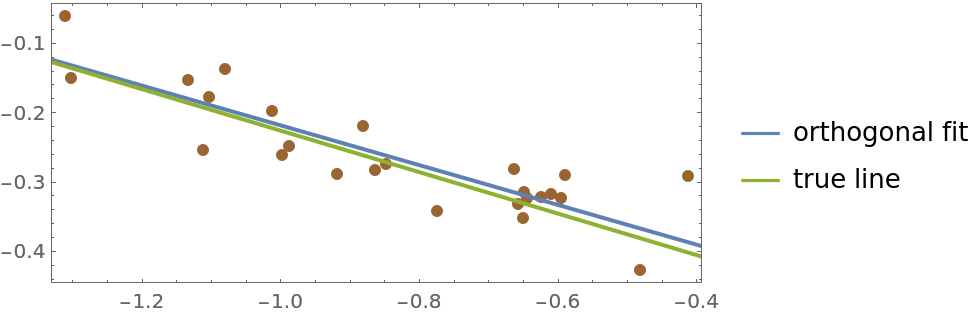 |
Parameters for a 3D line:
| In[5]:= | ![BlockRandom[SeedRandom[42, Method -> "ExtendedCA"];
{p0, v0} = {RandomReal[{-2, 2}, 3], Normalize[RandomVariate[NormalDistribution[], 3]]}]](https://www.wolframcloud.com/obj/resourcesystem/images/115/115b0475-c4a7-41e2-aca2-d63d90fe1a4c/0d18295e66dc107e.png) |
| Out[5]= |  |
Generate some points near the line:
| In[6]:= | ![BlockRandom[SeedRandom[42, Method -> "ExtendedCA"];
pts = Table[
p0 + t v0 + RandomVariate[NormalDistribution[0, 1/8], 3], {t, RandomReal[1, 25]}]]](https://www.wolframcloud.com/obj/resourcesystem/images/115/115b0475-c4a7-41e2-aca2-d63d90fe1a4c/54482d488aa09514.png) |
| Out[6]= |  |
Find the orthogonal distance regression line:
| In[7]:= | ![ofit = ResourceFunction["OrthogonalLineFit"][pts]](https://www.wolframcloud.com/obj/resourcesystem/images/115/115b0475-c4a7-41e2-aca2-d63d90fe1a4c/7a315b08b724ee30.png) |
| Out[7]= |  |
Compare the regression line and the true line with the data:
| In[8]:= | ![Legended[
Graphics3D[{{Directive[AbsolutePointSize[6], Brown], Point[pts]},
{Directive[AbsoluteThickness[2], ColorData[97, 1]], ofit},
{Directive[AbsoluteThickness[2], ColorData[97, 3]], InfiniteLine[p0, v0]}}, Axes -> True],
LineLegend[{ColorData[97, 1], ColorData[97, 3]}, {"orthogonal fit", "true line"}]]](https://www.wolframcloud.com/obj/resourcesystem/images/115/115b0475-c4a7-41e2-aca2-d63d90fe1a4c/34a09ef019dea07c.png) |
| Out[8]= | 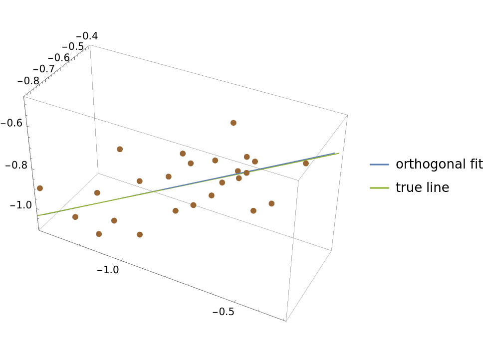 |
Here is a list of values:
| In[9]:= |  |
When coordinates are not given, OrthogonalLineFit assumes the values are to be paired up with 1,2,…:
| In[10]:= | ![ofit = ResourceFunction["OrthogonalLineFit"][v]](https://www.wolframcloud.com/obj/resourcesystem/images/115/115b0475-c4a7-41e2-aca2-d63d90fe1a4c/7841aaf57163a217.png) |
| Out[10]= |  |
| In[11]:= | ![ListPlot[v, Epilog -> {ColorData[97, 3], ofit}]](https://www.wolframcloud.com/obj/resourcesystem/images/115/115b0475-c4a7-41e2-aca2-d63d90fe1a4c/164f538df5ffc78e.png) |
| Out[11]= | 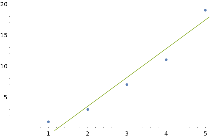 |
Here is some data:
| In[12]:= |  |
This computes the parameters for the orthogonal distance regression line using the definition:
| In[13]:= | ![{pm, vm} = Partition[
NArgMin[Total[
RegionDistance[InfiniteLine[{px, py}, {vx, vy}], #]^2 & /@ data], {px, py, vx, vy}], 2]](https://www.wolframcloud.com/obj/resourcesystem/images/115/115b0475-c4a7-41e2-aca2-d63d90fe1a4c/626393a089c9c390.png) |
| Out[13]= |  |
Use OrthogonalLineFit to get the best-fit line:
| In[14]:= | ![ofit = ResourceFunction["OrthogonalLineFit"][data]](https://www.wolframcloud.com/obj/resourcesystem/images/115/115b0475-c4a7-41e2-aca2-d63d90fe1a4c/6a66e8a830fbb5e7.png) |
| Out[14]= |  |
Use RegionMember to compare the equations for the best fit line generated by both methods:
| In[15]:= | ![Simplify[{RegionMember[InfiniteLine[pm, vm], {x, y}], RegionMember[ofit, {x, y}]}, {x, y} \[Element] Reals]](https://www.wolframcloud.com/obj/resourcesystem/images/115/115b0475-c4a7-41e2-aca2-d63d90fe1a4c/717f3c1ddac4f222.png) |
| Out[15]= |  |
Construct a function from the orthogonal fit:
| In[16]:= | ![oFun[x_] = Expand[y /. First[Solve[Last[%], y]]]](https://www.wolframcloud.com/obj/resourcesystem/images/115/115b0475-c4a7-41e2-aca2-d63d90fe1a4c/38ee6ce66fa921bc.png) |
| Out[16]= |  |
Compare the orthogonal fit with the conventional least-squares fit:
| In[17]:= | ![lFun[x_] = Fit[data, {1, x}, x]](https://www.wolframcloud.com/obj/resourcesystem/images/115/115b0475-c4a7-41e2-aca2-d63d90fe1a4c/1116e1e606d159cc.png) |
| Out[17]= |  |
| In[18]:= | ![Plot[{oFun[x], lFun[x]}, {x, 0, 5}, Epilog -> {Directive[AbsolutePointSize[4], ColorData[97, 4]], Point[data]}, PlotLegends -> {"orthogonal fit", "least-squares fit"}]](https://www.wolframcloud.com/obj/resourcesystem/images/115/115b0475-c4a7-41e2-aca2-d63d90fe1a4c/04597bf858a873c4.png) |
| Out[18]= | 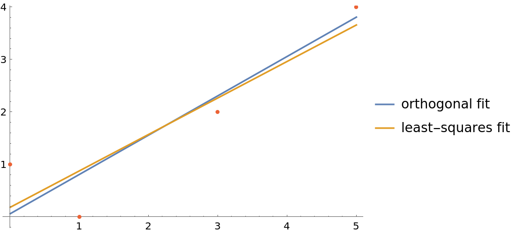 |
This work is licensed under a Creative Commons Attribution 4.0 International License
