This post starts with the the slides of an elementary talk I gave at Sloans Bar and Grill, in Glasgow, as part of a wonderful series called A Pint of Science. At the end I include some fascinating details which I only had time to briefly touch on in my talk. If you already know plenty of physics, this is the juicy stuff.

Start with a hair:

A red blood cell is ten times smaller across:

A flu virus is 10 times smaller across than that:

The flagellum of this cell is ten times smaller across than that:

A molecule of hemoglobin is about ten times smaller than that:

A water molecule is ten times smaller than that:

A hydrogen atom is 5 times smaller than that:

This is an actual image of a single hydrogen atom, which is amazing. (Read more here.)
But how did people figure out that atoms even exist, back before we could see individual atoms? And how did we figure out what they’re made of?
It started with chemistry. Two liters of hydrogen burn with one of oxygen to form one liter of water vapor, so we guess water is made of 2 atoms of hydrogen and 1 of oxygen: H2O. But one cubic meter of oxygen is 16 times heavier than one of hydrogen, so we guess O is 16 times heavier than H.
And so on — this took a lot of detective work, back in the 1800s.
By 1871, Mendeleev created the periodic table, listing atoms in order of weight. Here’s a modern version:
But what are the numbers on these elements? They are called atomic numbers. They are not the atom’s weights. Now we know it’s the number of electrons they have! But how did we find out about electrons?
In 1869, William Crookes made a beam by evacuating a glass tube and running an electric current though it:
In 1897, J. J. Thomson showed that this beam is made of particles less than one thousandth the mass of hydrogen atoms! We now call these particle electrons though Thomson disliked this term. (Read more here.)
Electrons are negatively charged, but atoms have no charge, so there must be something positively charged in the atom. Thomson proposed that an atom is a ball of positive charge with electrons speckled throughout it. A journalist called this the plum-pudding atom, and the name stuck. (Read more here.)
But in 1886, Eugen Goldstein created a beam moving in the opposite direction from the electrons in an evacuated tube! (Read more here.)
In 1898 Wilhelm Wien showed this beam is made of positively charged particles with about the same mass as a hydrogen atom. It took a long time to realize the full importance of these particle. We now call them protons. (Read more here.)
In 1909 Rutherford’s team in Manchester showed that the positive charge in an atom is concentrated in a small part near its center: the nucleus.
His assistants Geiger and Marsden fired particles (which we now know are helium nuclei) at some gold leaf, and some bounced back. When Rutherford saw the results of this experiment, he wrote “it was almost as incredible as if you had fired a 15-inch shell at a piece of tissue paper and it came back and hit you”. The plum-pudding model was out!
But there’s a big problem. The “atomic weight” is the little number at the bottom of each square here:
If protons account for almost all the mass of the atom, the atomic weight of an atom should be the number of protons it contains. But since the atomic weight is bigger than the atomic number, this would mean atoms would have more protons than electrons — hence be positively charged. They’re not!
Let’s not even worry now about the fact that the atomic weight is not always close to an integer. Let’s just worry about this: how could an atom have more protons than electrons, if it’s electrically neutral?
Here’s one possible solution: the nucleus contains extra electrons to cancel out the excess positive charge. Rutherford argued for this in 1920.
For example helium has atomic number 2, but atomic mass 4. With 2 electrons and 4 protons, helium would have charge +2. It doesn’t! But if it also had 2 extra electrons in the nucleus it would be neutral, as observed.
But what would make some of the electrons stay in the nucleus, while others orbit it?
In 1930, Marie Curie’s daughter Irène and her husband created a beam of electrically neutral particles by bombarding the metal beryllium
with radiation.
In Cambridge, James Chadwick carried these experiments further and proved there was a neutral particle with almost the same mass as a proton: the neutron. (Read more here.)
It became clear that the nucleus of an atom is made of protons and neutrons!
Later experiments showed a nucleus is about 1/60,000 as big across as an atom. If the hydrogen atom were a sphere 30 meters across, the proton would be a grain of salt at the center.
This raises another huge problem. If the protons are confined in the tiny nucleus, and they’re all positively charged, they must repel each other immensely! What holds them together?
But that’s another story! I’ve sketched out how we figured out the basics of atoms — that’s atomic physics. The next story would be nuclear physics. There are always new puzzles, leading us onward.
Digression: photographing a hydrogen atom
The photograph is not just a picture of the wavefunction of the electron in a hydrogen atom; it’s the result of a complicated process. For more try these:
The second is more careful than its title. It does the unusual and welcome thing of saying that “the experimentally observed nodal structures originate from the transverse nodal structure of the initial state that is formed upon laser excitation” — which is the actual claim, properly hedged, rather than “we photographed the orbital.” It also notes the comparison between measured and predicted images, which makes clear that this is a quantitative experiment with theory backing it, not a literal photograph.
Digression: J. J. Thomson
In fact, the man who discovered the electron through some of the most delicate vacuum-tube experiments ever performed was reportedly a complete disaster with his hands.
J. J. Thomson was hopeless in the lab. His assistant Ebenezer Everett forbade Thomson from touching anything delicate on the grounds that he was “exceptionally helpless with his hands”. According to Ainissa Ramirez:
For such a small man, he was a Victorian bull in a china shop. When he visited his students in the laboratory, they’d wince when he offered help, and quickly tried to move fragile things out of his way. They took deep breaths when he sat on a lab stool to speak. Life was no better at home. J. J.’s wife did not permit him to use a hammer in the house.
The irony: the 1897 electron experiments depended absolutely on glassware that almost no one in the world could make. You needed cathode-ray tubes capable of holding a vacuum so high that any ordinary tube would shatter, with metal electrodes sealed through the glass without leaking. Everett, a self-taught glassblower who had migrated over from the chemistry department, made every tube by hand. Thomson didn’t touch them.
Thomson called the particles he discovered “corpuscules”. The word “electron” was already in circulation when he made his announcement: George Johnstone Stoney had coined it in 1891 for the unit of charge in electrolysis, and Joseph Larmor was already using it in 1894 for a theoretical particle in his electromagnetic ether theory. Within months of Thomson’s April 1897 lecture, George FitzGerald suggested that the corpuscle identified by Thomson from cathode rays and proposed as parts of an atom was a “free electron,” as described by physicist Joseph Larmor and Hendrik Lorentz. While Thomson did not adopt the terminology, the connection convinced other scientists that cathode rays were particles.
Thomson dug in. He kept saying “corpuscle” through the whole period when he was actually building his case for the particle — the 1899 paper showing the photoelectric particles had the same m/e, the 1904 plum-pudding model paper, the 1906 Nobel Prize, all discussed “corpuscles.” Thomson himself continued to use the term corpuscle until 1913 — about sixteen years after his announcement, and well after the rest of the physics community had moved on. His 1906 Nobel citation reflects how oddly Thomson’s contribution was framed at the time: “His 1906 Nobel Prize was granted ‘in recognition of the great merits of his theoretical and experimental investigations on the conduction of electricity by gases,’ not for any specific discovery, let alone the electron (which he kept calling the corpuscle)”.
Part of the resistance was substantive, not just stubborn. “Electron” in Larmor’s and Lorentz’s usage was a theoretical entity tied to an ether-based electromagnetic worldview, with specific commitments Thomson didn’t want to inherit. Calling his thing a “corpuscle” let him keep it as a mechanical, material particle — a building block of the atom in his own picture — without buying into the Continental electromagnetic program.
So the textbook line “Thomson discovered the electron in 1897” smooths over a real conceptual identification that took a decade and a half, and that Thomson himself was among the last to embrace.
For more, try:
• Isobel Falconer, Corpuscles to electrons in Histories of the Electron, Buchwald and Warwick, eds., MIT Press, Cambridge, 2001.
• Ainissa Ramirez, The Alchemy of Us—How Humans and Matter Transformed One Another, MIT Press, Cambridge, Massaschusetts, 2020.
Digression: the plum-pudding atom
The “plum pudding” name was invented by an anonymous popular-science writer in 1906. You can see a careful historical reconstruction here:
• Giora Hon and Bernard R. Goldstein, J. J. Thomson’s plum-pudding atomic model: the making of a scientific myth, Annalen der Physik 525 (2013), A129–A133.
Hon and Goldstein tracked down the earliest occurrence: an anonymous reporter in the British pharmaceutical trade magazine The Chemist and Druggist, August 1906, who described the atom as having “minute specks, the negative corpuscles, swimming about in a sphere of positive electrification, like raisins in a parsimonious plum-pudding”. “The analogy was never used by Thomson nor his colleagues. It seems to have been coined by popular science writers to make the model easier to understand for the layman.”
In fact, by the time the Chemist and Druggist writer reached for the pudding image in 1906, Thomson’s model had already moved past the version it was supposedly describing. As Hon and Goldstein put it: “according to Thomson’s theory of 1906, the electrons revolve on rings about the center of the atom, and they are not distributed throughout the ‘pudding’ as ‘raisins swimming about.'” The pudding image was obsolete from the moment it was coined.
What Thomson actually used as his guiding analogy was much more interesting: floating magnets. Thomson drew an analogy with experiments by Alfred Marshall Mayer (1836–1897). Piercing small magnetic needles into corks and letting them float in water below a strong magnet, Mayer had observed in 1878/79 that the magnetized floating needles quasi-automatically positioned themselves in characteristic configurations depending on their number. With more than six magnetic needles present, a seventh and eighth would inevitably position itself inside the outer ring of six. As the number of floating magnets increased, more and more rings would form. Thomson hoped that a similar ring-structure composed of corpuscles could be found inside chemical atoms, and suspected that each of these rings would be analogous to the chemical periods. So in Thomson’s head, the atom looked like Mayer’s needle-in-cork rings — dynamic, self-organizing, suggestive of the periodic table, not a dessert.
Another question: was the model even Thomson’s alone? Britannica notes that the model was “proposed about 1900 by William Thomson (Lord Kelvin) and strongly supported by Sir Joseph John Thomson, who had discovered (1897) the electron”. Kelvin had been working on similar uniform-positive-sphere ideas a few years before J.J. Thomson’s 1904 Philosophical Magazine paper, so the standard “Thomson’s plum pudding” of textbooks elides both a co-originator and the actual originator of the name.
• A. M. Mayer, Floating magnets, Nature 17 (1878), 487–488.
• Klaus Hentschel, Atomic Models, J.J. Thomson’s ‘Plum Pudding’ Model, in Compendium of Quantum Physics, eds. D. Greenberger, K. Hentschel and F. Weinert, Springer, Berlin, 2009.
• John Heilbron, J.J. Thomson and the Bohr atom, Physics Today 30 (1977), 23–30.
• Wikipedia, Plum pudding model.
• Britannica, Thomson atomic model.
Digression: Eugen Goldstein
In Crookes’ tube, electrons flew from a negatively charged metal tip (the cathode) to the positively charged one (the anode). Thus, electrons were called cathode rays, and this apparatus was called a cathode ray tube.
By the mid-1880s, the phenomena created by these tubes was a hot but baffling field. There was a vigorous debate about whether cathode rays were charged particles (the Crookes/Schuster view) or some kind of wave in the aether (the German view, which Goldstein himself leaned toward). In 1876, Goldstein discovered that cathode rays were emitted perpendicular to the cathode surface. This inspired the design of concave cathodes to produce concentrated or focused rays. So experimenters were routinely fiddling with cathode geometries — different shapes, different sizes, different configurations — to study cathode ray behavior. Goldstein spent his time doing this.
Eventually, around 1886, he tried drilling small holes in the cathode — Kanäle, meaning “channels” or “canals”. He discovered something surprising: wth the tube running, a faint glow appeared streaming out the back of the cathode, opposite to the direction of the cathode rays. Busch writes: “Goldstein therefore called them ‘canal rays’ (German ‘Kanalstrahlen’). Since the canal rays went in the opposite direction as the ‘cathode rays’, Goldstein speculated that these rays consisted of positively charged particles.”
Later these canal rays were called “anode rays” as a parallel to “cathode rays,” but it’s somewhat misleading — these rays don’t actually originate at the anode. They “are produced by positively charged ions after impact ionization in the cathode ray tubes. These ions are accelerated towards the cathode, pass — if the cathode is provided with holes — through these holes (‘channels’) due to their inertia and can be detected behind the cathode by their luminous phenomena.” So they’re lone protons formed in the gas, accelerated toward the cathode, that shoot through the holes by inertia and emerge on the far side.
• Britannica, Eugen Goldstein.
• Wikipedia, Eugen Goldstein.
• Encyclopedia of Scientific Biography, Eugen Goldstein.
• Uwe Busch, Claims of priority — The scientific path to the discovery of X-rays, Z. Med. Phys. 19 (2023), 230–242.
Digression: Wilhelm Wien
Wilhelm Wien, famous for his work on blackbody radiation, was working at Aachen when in 1898 he turned to the problem Goldstein had left dangling. Goldstein himself had tried to deflect canal rays magnetically and failed. Using the strongest magnet he had, one that certainly had an effect on the cathode rays, Goldstein attempted to deflect his canal rays, but he observed no change in their path. So for twelve years the rays were a sort of mystery — clearly something real, but resistant to the magnetic deflection trick that was the standard probe of the era.
Wien managed to bend canal ways using brute force. To deflect the cathode rays, you only needed a modest field. To deflect the canal rays, Wien needed a magnetic field of 3250 gauss and a electrical field of 2000 V — and his rays moved a grand total of 6 mm. The thing was enormously more sluggish to deflect than electrons, and this meant the particles were vastly more massive per unit charge. Goldstein hadn’t been doing anything wrong — he just hadn’t been hitting them hard enough!
The really nice piece of physics is how Wien figured out the charge/mass ratio of canal rays. He invented what we now call the Wien filter: a charged-particle velocity filter with orthogonal electric and magnetic fields. The trick is elegant. The magnetic force on a particle depends on its velocity; the electric force doesn’t. So if you tune the fields against each other, only particles of one particular velocity sail straight through undeflected — everything else gets bent. Once you know the velocity, the deflection in a pure magnetic field tells you charge-to-mass. It’s a beautiful idea, and it’s still the working principle behind ion-beam instruments today.
Wilhelm Wien analyzed these positive rays in 1898 and found that the particles have a mass-to-charge ratio more than 1,000 times larger than that of the electron. Because the ratio of the particles is also comparable to the mass-to-charge ratio of the residual atoms in the discharge tubes, scientists suspected that the rays were actually ions from the gases in the tube. So Wien did not discover the proton, contrary to what’s sometimes claimed. What he found was:
• The deflection was in the opposite direction from cathode rays — so the particles were positively charged.
• The charge-to-mass ratio depended on the gas in the tube, not on the cathode material — so these weren’t some universal particle like the electron; they were ions of whatever gas you’d filled the tube with.
• The mass-to-charge ratio was comparable to atomic masses, meaning these were essentially atoms missing electrons.
The hydrogen ion — which we now call the proton — was just one of many ions Wien could produce, and there was nothing special about it in his work. The identification of the hydrogen ion as a fundamental constituent of all nuclei came much later, with Rutherford’s nuclear-scattering experiments and his 1919 demonstration that he could knock hydrogen nuclei out of nitrogen. Rutherford named it the proton around 1920.
So the lineage is this: Goldstein 1886 saw a glow, Wien 1898 showed it was ionized gas, and finally Rutherford 1919–1920 identified the hydrogen ion as a universal nuclear building block.
Digression: Discovery of the neutron
The discovery of the neutron was an extremely complicated business, starting with the the problem of understanding atomic mass (Z) and atomic number (A) in the periodic table.
Prout, isotopes, and the Z-vs-A puzzle. The puzzle has roots in William Prout’s 1815 hypothesis that atomic weights are integer multiples of hydrogen, suggesting hydrogen as a building block for all the other elements. Through the nineteenth century this looked broken: chlorine sat at 35.5, and most elements were not clean integers. Two developments rehabilitated it. Soddy in 1913 introduced the concept of isotopes — the same element can exist in chemically identical forms of different mass — explaining the non-integer atomic weights as weighted averages. J.J. Thomson’s 1912–13 work on neon gave the first stable-element example, and Aston’s mass spectrograph (1919 onwards) established what Aston called the “whole-number rule”: individual isotopes have atomic masses very nearly integral in units of hydrogen, with small deviations here and there. In parallel, Moseley’s 1913 work using X-rays pinned down atomic number Z as the nuclear charge, not just an ordinal label. Putting these together you got the central puzzle: for elements heavier than hydrogen, the atomic mass A is larger than the atomic number Z!
The proton-electron nucleus. The obvious move was: maybe the nucleus contains A protons and A − Z electrons, giving the right charge and mass. The model was appealing on three grounds beyond accounting. First, only two particles were known (proton and electron), so parsimony favored it. Second, beta decay does eject electrons from nuclei, so the electrons appeared to be there to begin with. Third, alpha particles (helium-4 nuclei) could be assembled as 4p + 2e, neatly. Rutherford himself adopted this picture in his 1920 Bakerian Lecture:
• Ernest Rutherford, Nuclear constitution of atoms, Proc. Roy. Soc. A 97 (1920), 374–400.
In that lecture he went further: he proposed that some proton-electron pairs inside the nucleus might be bound so tightly as to form a compact neutral unit: “the idea of the possible existence of an atom of mass one, which has a zero nuclear charge”. He floated the term “neutron” for it. (W.D. Harkins coined the same term independently in 1921.) Note that Rutherford’s neutron was not a new elementary particle; it was a compound, a sort of miniature hydrogen atom. This conception persisted for over a decade and shaped how the discovery was eventually interpreted.
Three killer problems with electrons in the nucleus. Through the 1920s, three independent objections accumulated.
• The confinement problem. Confining an electron to a nucleus of radius ~10⁻¹⁴ m gives, by the uncertainty principle, a momentum spread of order ℏ/r and hence a kinetic energy of order ~20 MeV — far larger than any nuclear binding energy then known, and far larger than the energies of beta-decay electrons. With Dirac’s relativistic electron theory (1928), things got worse: Klein’s paradox showed that electrons in sufficiently strong potentials don’t bind cleanly at all. Bohr was so disturbed by this that around 1929–30 he was openly speculating that energy and momentum conservation might fail at nuclear scales.
• The nitrogen-14 anomaly. This is the cleanest of the three and the one that broke the model. Studies of the spectrum of molecular nitrogen in the late 1920s showed that the nitrogen-14 nucleus is a boson, hence must have integer spin. (Direct measurement gave spin 1.) But in the theory where a neutron is a proton-electron combination model, nitrogen-14 would be 14p + 7e = 21 spin-½ fermions, which must have half-integer total spin and thus be a fermion. The model predicted the wrong thing for the most common nitrogen isotope!
• The continuous beta spectrum. Chadwick himself, back in 1914, had shown that beta decay produces a continuous energy spectrum, not a line spectrum. Ellis, Wooster, and (decisively) Meitner and Orthmann’s 1929 calorimetric experiment confirmed energy was apparently not conserved. Pauli’s famous December 1930 letter “Dear Radioactive Ladies and Gentlemen” proposed a neutral, spin-½, light particle inside the nucleus to fix both energy conservation and the spin-statistics problem simultaneously — he called his particle a “neutron” too. (Fermi renamed it “neutrino” in 1933 after Chadwick’s discovery, to avoid the name collision.)
So by 1930 there were three structurally independent reasons to think the proton-electron nucleus was wrong, and Rutherford had a candidate replacement that nobody had yet found.
The 1930–32 experimental crescendo. The discovery story is what the Encyclopedia of Scientific Biography calls a “Tale of Three Cities” — Berlin, Paris, and Cambridge. “Walther Bothe and his assistant Herbert Becker [were] working in the Physikalisch-Technische Reichsanstalt (Imperial Physical-Technical Institute) in Charlottenburg, a suburb of Berlin; Irène Curie and her husband Frédéric Joliot working in the Institut du Radium in Paris; and James Chadwick working in the Cavendish Laboratory in Cambridge. The story reached its crescendo between June 1930 and February 1932.”
• Berlin, 1930. Walther Bothe and Herbert Becker observed that bombarding beryllium with alpha particles emitted a highly penetrating, electrically neutral radiation. They, along with most of the scientific community, incorrectly assumed this radiation was exceptionally high-energy gamma rays. Lead absorption coefficients suggested gamma rays of unprecedented energy — odd, since the nuclear binding energies available from α + ⁹Be shouldn’t have been enough.
• Paris, late 1931 – January 1932. Irène Joliot-Curie and Frédéric Joliot, with the world’s strongest polonium alpha source (an inheritance, essentially, from Marie Curie’s lab), pushed the Bothe radiation through a paraffin window. They found that this radiation knocked loose protons from hydrogen atoms in that target, and those protons recoiled with very high velocity. They interpreted the result as the scattering of high-energy photons off protons — which, as Chadwick noted in his Feb 27, 1932 Nature letter, required “that the beryllium radiation had a quantum energy of 50 × 10⁶ electron volts”. That was about ten times more energy than any plausible nuclear gamma source could produce. Curie and Joliot reported their findings on 18 January 1932, and the Comptes Rendus arrived in Cambridge within a couple of weeks.
• Cambridge, February 1932. Chadwick read the paper and, primed by Rutherford’s 1920 prediction and his own decade-long search for the neutron, instantly suspected the right answer. Rutherford’s reported reaction was characteristic: “I do not believe it!” Chadwick built the experiment immediately — borrowed polonium, the Cavendish’s beryllium, an ionization chamber. The crucial idea was simply to substitute multiple other targets for the paraffin: hydrogen, nitrogen, helium, lithium. If the projectile is a massive neutral particle of unknown mass m, you can work out the maximum recoil velocity of a nucleus of mass M. Comparing the maximum recoil velocities for hydrogen and nitrogen, Chadwick could solve algebraically for m. He found m is close to the proton mass. Three weeks after reading the Paris paper, he submitted a paper on the possible existence of a neutron on February 17th, 1932, which was published ten days later:
• James Chadwick, Possible existence of a neutron, Nature 129 (1932), 312.
He sent a fuller, more confidently titled paper to the Royal Society on the 10th of May:
• Chadwick, The existence of a neutron, Proc. Roy. Soc. A 136 (1932), 692–708.
Aftermath: from compound to elementary. Chadwick himself, in 1932, still followed Rutherford and described the neutron as a tight proton-electron compound — he wasn’t yet claiming a new elementary particle. The shift came over the next two years. Heisenberg’s three “On the structure of atomic nuclei” papers (July–December 1932) treated the proton and neutron as two states of a single ‘nucleon’ with the strong force coupling them via isospin — a structure that doesn’t work at all if the neutron has an electron lurking inside it. Fermi’s January 1934 theory of beta decay treated the electron as created at the moment of decay (the electromagnetic-radiation analogy: photons aren’t “in” the atom before emission either), removing the last motivation to put electrons in the nucleus. And the final empirical nail, suggested to Chadwick by the young Maurice Goldhaber, was photodisintegration of the deuteron: γ + d → p + n. By energy conservation, the neutron mass came out at greater than 1.0077 and less than 1.0086 in atomic mass units. Thus, the neutron was more massive than the hydrogen atom which had an accurately determined mass of 1.0078 amu. A bound p+e would weigh less than free p plus free e (binding energy is negative); since the neutron weighs more than a hydrogen atom, it cannot be such a bound state. By 1934 the neutron was firmly an elementary particle.
Primary sources and good histories:
• Lawrence Rutherford, Bakerian Lecture: nuclear constitution of atoms, Roy. Soc. Proc. A 97 (1920), 374–400.
• Irène Joliot-Curie and Frédéric Joliot-Curie, Émission de protons de grande vitesse par les substances hydrogénées sous l’influence des rayons γ très pénétrants, Comptes Rendus 194 (1932): 273.
• APS News, Chadwick reports the discovery of the neutron, May 1932.
• S. M. Bilenky, Neutrino: history of a unique particle.
• Roger Stuewer, The nuclear electron hypothesis, in Otto Hahn and the Rise of Nuclear Physics, Reidel, 1983.


 Posted by John Baez
 Taking logs we see

 This constant is called the
  which is defined by


 is the
  is the Riemann zeta function. By the way, this formula shows that calling
  a fancier relative of
  is not just talk.
 and the agreement is very good:


 by
by  in all the formulas, we get the
 which is called Galois conjugation. This is mentioned near the end of this book:
 be the
 rational, equipped with the usual addition, multiplication, subtraction and division. Define Galois conjugation


 :
:


 whose vertices lie in
  Beware: such a pentagon is impossible in the plane!
 coordinatewise; let’s abuse language and call this map
 be the vertices of a regular pentagon, listed in cyclic order. Then
  listed in the same cyclic order, are the vertices of a regular pentagram.

 so this is the angle between the consecutive edge vectors
  and
and  Since
Since

 and
and  It is easy to check that the usual dot product of
  obeys
obeys


 is
is


 is positive, because we claimed that the usual positive square root of
  equals
  and we also felt free to divide by
  Why is
 we have

 is injective, so the
  are not all zero.
 are coplanar, since coplanarity amounts to the vanishing of certain 3 × 3 minors in the matrix of coordinate differences, which is a polynomial condition over
  hence preserved by
  These points are also distinct, since
  thus form a planar closed
  -gon with equal edge lengths
  and constant exterior turning angle
  at each vertex. This is a regular pentagram. █
 we get back a regular pentagon. And if you’re worried about what happened to the plane, fear not! We can draw regular pentagons in the plane whose vertices have coordinates in a certain quadratic extension of
  This larger field again has an automorphism that carries regular pentagons to regular pentagrams.


 the pentagons turn into pentagrams, while the squares stay squares and the equilateral triangles stay equilateral triangles. It gets messy if we draw everything, but if we draw just the pentagrams it’s beautiful:
 so they change as they become pentagram edges.


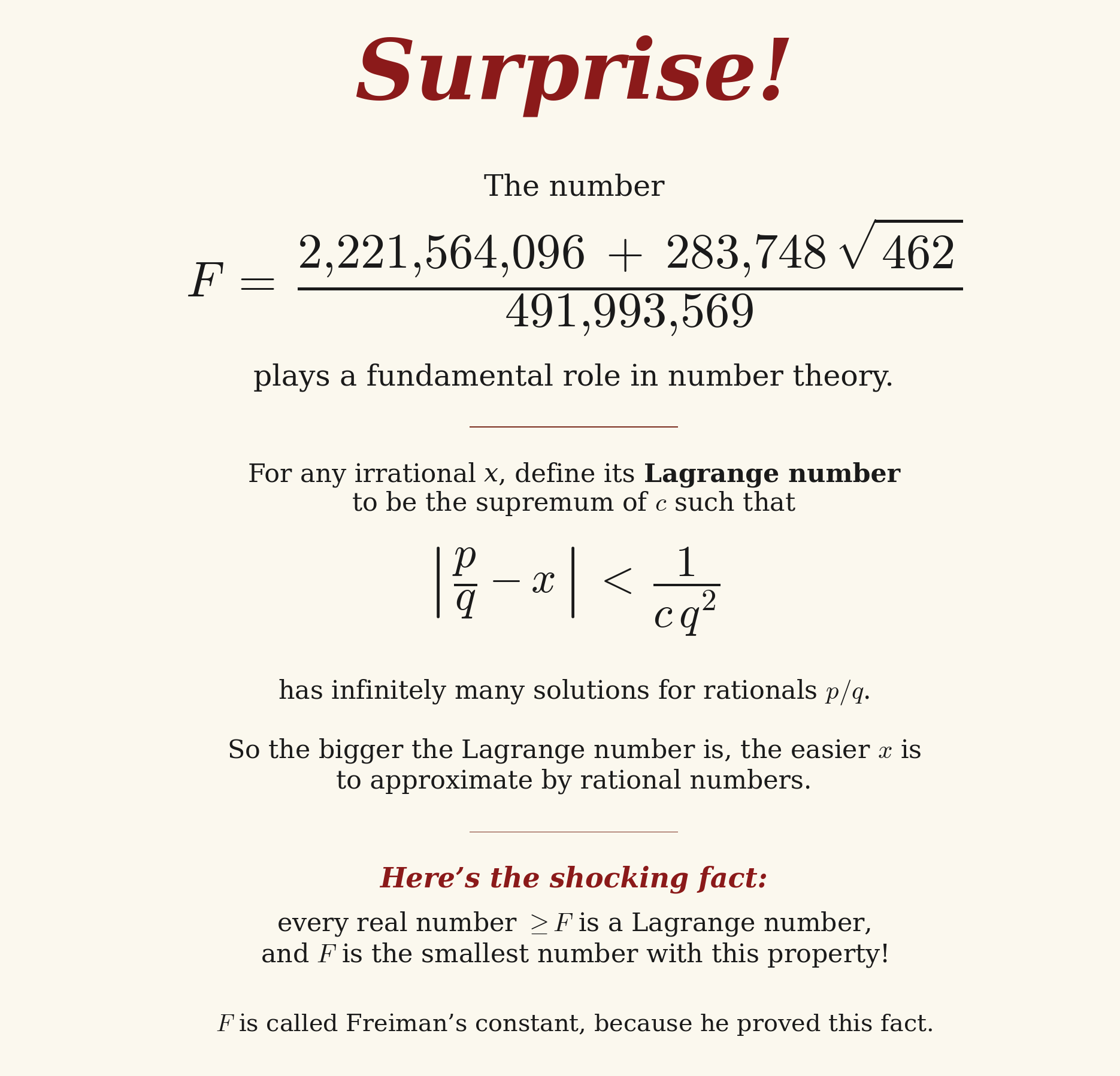

 we define its Lagrange number to be the supremum of numbers
  such that
 So, the easier
  is to approximate by rational numbers, the bigger its Lagrange number is.
 is a Lagrange number, and
  is the smallest number with this property!
 The next is
  The next is
  In 1879, Markov showed that such numbers form an increasing sequence that converges to 3. They are precisely the Lagrange numbers of numbers whose continued fraction expansion and eventually consists only of 1’s and 2’s and is eventually periodic, like this:
 the Hausdorff dimension of the Lagrange spectrum hits 1. And as mentioned, Freiman showed that above


 because the particle simply disappears when it hits the origin. Here we focus on theories where time evolution is unitary and the particle comes back out. Many people have written about these, running into ‘paradoxes’ when they weren’t careful enough. Only rather recently have things been straightened out.
 is
is  In a central force whose strength is proportional to
  such a particle has a Hamiltonian of this form:
 to remove irrelevant clutter, but we need the constant
  the force is attractive.
 as a densely defined linear operator on
  and treat
  to
to  and a linear operator
  to
to  we define
  to be the set of all
  for which there exist
  such that
 exists, it is unique, and it depends linearly on
  Thus, for
  we define
  to be the vector
  We say
  We say that
 In this case we can start with the domain
  consisting of smooth functions that are compactly supported on
  In this case
  but it is not essentially self-adjoint. In fact, it admits more than one self-adjoint extension! However,
  such that
 Physically, this means that the particle’s energy is bounded below by
  Mathematically, this implies that
  In this case
  ? In classical mechanics, the energy of a particle in the inverse cube force ceases to be bounded below as soon as
  Quantum mechanics is different. To get a lot of negative potential energy, the particle’s wavefunction must be peaked near the origin, but that gives it kinetic energy. The tradeoff is captured by Hardy’s inequality. This says that for any
  we have

 in Hardy’s inequality cannot be improved, so if
  we can find
  with
with  Then we can use a remarkable property of the
  potential to show that
  dilate it by a factor of
  and then apply
  you get
  times what you get if you do these operations in the other order. This implies that if
 replaced by
  Thus, as soon as
  to be very small. Thus
  ? This is more subtle. For any value of
  we can find spherically symmetric solutions of
 that are nonzero and smooth. When
  and only in this case, some of these solutions
  If
If  would be self-adjoint, and it is easy to see that a self-adjoint operator cannot have
  as an eigenvalue.
 the operator
  as a sum of a radial part and an angular part, assuming the angular dependence of
  and doing a change of variables
  to reduce
 We can completely classify self-adjoint extensions of this differential operators from
  to larger domains; the answer depends on
  A choice of self-adjoint extension is a choice of boundary conditions at
  and this says how the phase of an incoming wave changes as it reflects off the origin and bounces back. Finally, we can assemble the results for different spherical harmonics to classify self-adjoint extensions of
 the extension must break the dilation symmetry discussed above. This is what physicists call an ‘anomaly’: a symmetry of a classical system that fails to be a symmetry of the corresponding quantum system. But intriguingly, for some still lower values of

.png)