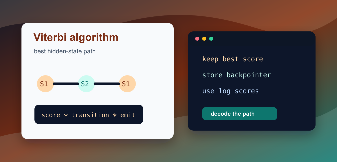
Viterbi Algorithm in Python: Dynamic Programming and Backpointers

Quick answer: The Viterbi algorithm uses dynamic programming to find the highest-scoring hidden-state path for an observation sequence. Store the best score per state and time step, keep backpointers, and use log probabilities when products would underflow.

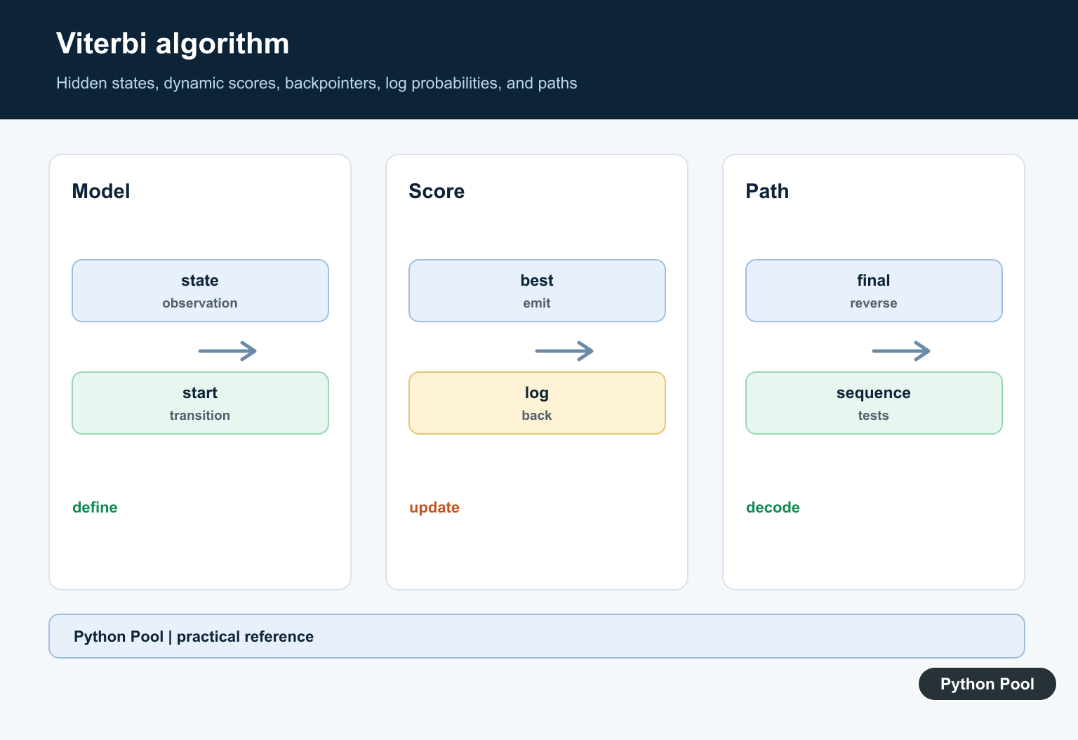
Python Pool infographic showing the Viterbi algorithm tracking best hidden-state scores and backpointers across an observation sequence — Viterbi keeps the best score for each hidden state at each time step and stores a backpointer so the most likely path can be reconstructed.

The Viterbi algorithm finds the most likely hidden-state path for an observed sequence. It is often used with hidden Markov models for tagging, speech recognition, spelling correction, signal processing, and other sequence tasks where each observed item depends on an unseen state.

A brute-force search would test every possible state path. That becomes expensive fast because each new observation multiplies the number of paths. Viterbi keeps only the best path ending in each state at each step, then extends those winners. This is dynamic programming: reuse the best partial results instead of recomputing every path.

Useful references for this guide include the Viterbi algorithm overview, Python’s math module, the tutorial section on dictionaries, and the max() function.

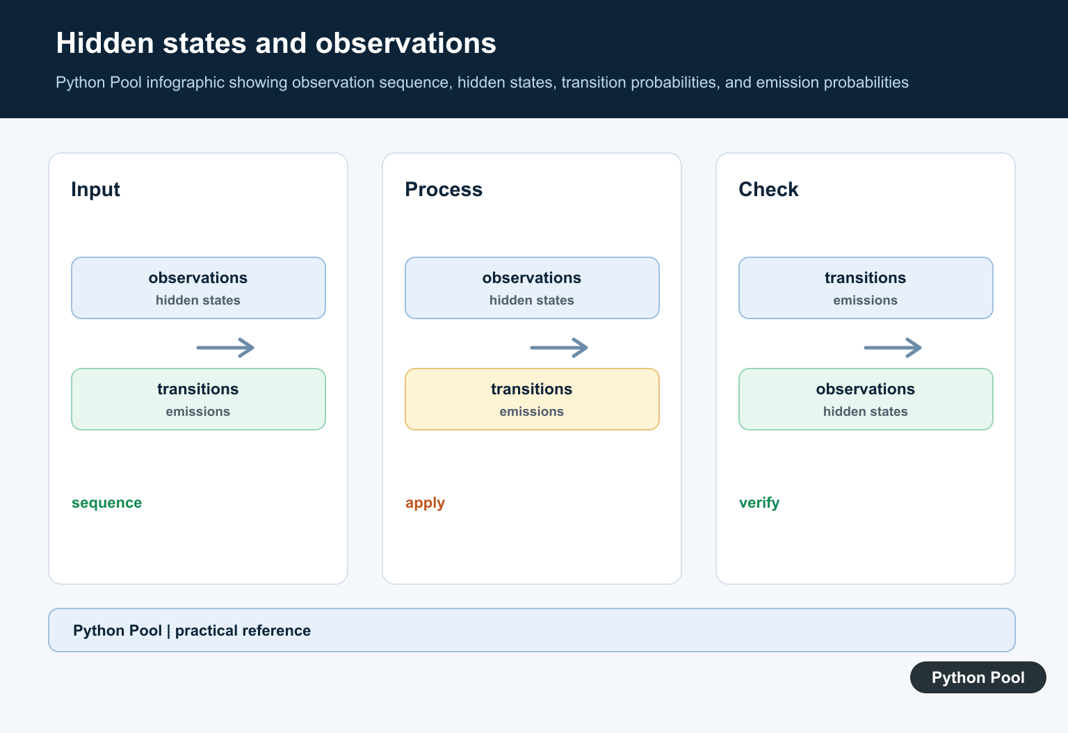
A Viterbi implementation needs four inputs: a list of possible states, the observed sequence, start probabilities, transition probabilities between states, and emission probabilities from states to observations. The output is the single most likely hidden-state path.

Contents

Score The First Observation

The first step combines the probability of starting in a state with the probability that the state emits the first observation. This creates the first column of the dynamic-programming table.

states = ["Rainy", "Sunny"]
observations = ["walk", "shop", "clean"]

start = {"Rainy": 0.6, "Sunny": 0.4}
emit = {
    "Rainy": {"walk": 0.1, "shop": 0.4, "clean": 0.5},
    "Sunny": {"walk": 0.6, "shop": 0.3, "clean": 0.1},
}

first = observations[0]
for state in states:
    score = start[state] * emit[state][first]
    print(state, round(score, 3))

The state with the highest first score is only the best local answer for the first observation. The full algorithm still needs transitions, because a slightly weaker start can lead to a stronger complete path.

Build A Complete Viterbi Function

The core loop keeps a score and path for each current state. For each next observation, it tests every previous state that could transition into the current state and keeps the best candidate.

def viterbi(states, observations, start, transition, emit):
    scores = {state: start[state] * emit[state][observations[0]] for state in states}
    paths = {state: [state] for state in states}

    for seen in observations[1:]:
        next_scores = {}
        next_paths = {}

        for state in states:
            previous, score = max(
                (
                    (old_state, scores[old_state] * transition[old_state][state] * emit[state][seen])
                    for old_state in states
                ),
                key=lambda item: item[1],
            )
            next_scores[state] = score
            next_paths[state] = paths[previous] + [state]

        scores = next_scores
        paths = next_paths

    best_state = max(scores, key=scores.get)
    return paths[best_state], scores[best_state]

states = ["Rainy", "Sunny"]
observations = ["walk", "shop", "clean"]
start = {"Rainy": 0.6, "Sunny": 0.4}
transition = {"Rainy": {"Rainy": 0.7, "Sunny": 0.3}, "Sunny": {"Rainy": 0.4, "Sunny": 0.6}}
emit = {"Rainy": {"walk": 0.1, "shop": 0.4, "clean": 0.5}, "Sunny": {"walk": 0.6, "shop": 0.3, "clean": 0.1}}

print(viterbi(states, observations, start, transition, emit))

This version returns both the path and its probability. It is small enough for teaching, but it still shows the real recurrence: previous score times transition probability times emission probability.

Python Pool infographic showing observation sequence, hidden states, transition probabilities, and emission probabilities — The Viterbi algorithm finds the most likely hidden-state path for an observed sequence.

Store Backpointers Instead Of Full Paths

For longer sequences, storing full paths at every step wastes memory. A common implementation stores only scores and backpointers, then reconstructs the best path at the end.

states = ["Noun", "Verb"]
words = ["fish", "swim"]
start = {"Noun": 0.7, "Verb": 0.3}
transition = {"Noun": {"Noun": 0.2, "Verb": 0.8}, "Verb": {"Noun": 0.6, "Verb": 0.4}}
emit = {"Noun": {"fish": 0.8, "swim": 0.1}, "Verb": {"fish": 0.2, "swim": 0.9}}

scores = [{state: start[state] * emit[state][words[0]] for state in states}]
back = []

for word in words[1:]:
    column = {}
    pointers = {}
    for state in states:
        previous, score = max(
            ((old, scores[-1][old] * transition[old][state] * emit[state][word]) for old in states),
            key=lambda item: item[1],
        )
        column[state] = score
        pointers[state] = previous
    scores.append(column)
    back.append(pointers)

print(scores[-1])
print(back)

A backpointer table records which previous state led to the best score for the current state. This is the standard shape used in many production implementations.

Use Log Scores For Long Sequences

Multiplying many small probabilities can underflow toward zero. Log scores replace multiplication with addition while preserving the same best-path decision.

import math

def log_value(number):
    return math.log(number) if number > 0 else float("-inf")

states = ["Hot", "Cold"]
observations = ["small", "large", "small"]
start = {"Hot": 0.5, "Cold": 0.5}
transition = {"Hot": {"Hot": 0.6, "Cold": 0.4}, "Cold": {"Hot": 0.3, "Cold": 0.7}}
emit = {"Hot": {"small": 0.2, "large": 0.8}, "Cold": {"small": 0.7, "large": 0.3}}

scores = {state: log_value(start[state]) + log_value(emit[state][observations[0]]) for state in states}
for seen in observations[1:]:
    scores = {
        state: max(scores[old] + log_value(transition[old][state]) + log_value(emit[state][seen]) for old in states)
        for state in states
    }

print({state: round(score, 3) for state, score in scores.items()})

Because logarithms are monotonic, the largest log score points to the same path as the largest normal probability. The numbers are also easier to keep stable for long inputs.

Handle Unknown Observations

Real data may contain an observation not listed in the emission table. A small fallback probability lets the algorithm continue while still penalizing the unknown item.

def emission_score(emit, state, seen, fallback=1e-6):
    return emit[state].get(seen, fallback)

states = ["Inside", "Outside"]
observations = ["dry", "windy"]
start = {"Inside": 0.55, "Outside": 0.45}
transition = {"Inside": {"Inside": 0.8, "Outside": 0.2}, "Outside": {"Inside": 0.3, "Outside": 0.7}}
emit = {"Inside": {"dry": 0.7}, "Outside": {"dry": 0.2}}

scores = {state: start[state] * emission_score(emit, state, observations[0]) for state in states}
seen = observations[1]
scores = {
    state: max(scores[old] * transition[old][state] * emission_score(emit, state, seen) for old in states)
    for state in states
}

print(scores)

The fallback should be chosen deliberately. Too high and unknown observations dominate the result; too low and every path becomes almost zero. In many models, smoothing is learned from training data.

Python Pool infographic showing time steps, state scores, best predecessor pointers, and Viterbi table — Store the best score for each state and time along with the predecessor that produced it.

Apply Viterbi To A Tiny Tagger

The same pattern works for a small part-of-speech tagger. The words are observations, and the hidden states are tags. The tiny example below repeats the decoder so the snippet can run by itself in a notebook, terminal, or test file.

def viterbi(states, observations, start, transition, emit):
    scores = {state: start[state] * emit[state][observations[0]] for state in states}
    paths = {state: [state] for state in states}

    for seen in observations[1:]:
        next_scores = {}
        next_paths = {}
        for state in states:
            previous, score = max(
                ((old, scores[old] * transition[old][state] * emit[state][seen]) for old in states),
                key=lambda item: item[1],
            )
            next_scores[state] = score
            next_paths[state] = paths[previous] + [state]
        scores = next_scores
        paths = next_paths

    best_state = max(scores, key=scores.get)
    return paths[best_state], scores[best_state]

tags = ["Noun", "Verb"]
sentence = ["time", "flies"]

start = {"Noun": 0.8, "Verb": 0.2}
transition = {"Noun": {"Noun": 0.1, "Verb": 0.9}, "Verb": {"Noun": 0.6, "Verb": 0.4}}
emit = {"Noun": {"time": 0.7, "flies": 0.2}, "Verb": {"time": 0.1, "flies": 0.8}}

path, score = viterbi(tags, sentence, start, transition, emit)

for word, tag in zip(sentence, path):
    print(word, tag)
print(round(score, 4))

A real tagger would learn start, transition, and emission probabilities from labeled text, then apply the same decoding process to new sentences. The table sizes change, but the recurrence is the same: score every possible previous state, keep the best predecessor, and continue to the next word.

When testing your own implementation, use a short hand-checkable sequence before trying a full dataset. Confirm the first column, one transition step, the final best score, and the reconstructed path. These small checks catch most mistakes in table indexing, missing emissions, and reversed transition keys.

In short, a Viterbi algorithm in Python needs clear probability tables, a recurrence that keeps the best previous state, and a way to reconstruct the final path. For small examples, normal probabilities are readable. For long sequences, use log scores and backpointers so the implementation stays stable and memory-efficient.

Define The Model

Specify hidden states, observations, initial probabilities, transition probabilities, and emission probabilities. Validate that rows and columns use the same state order throughout the calculation.

Python Pool infographic showing final best state, backpointers, reverse traversal, and decoded state sequence — Backpointers reconstruct the highest-scoring path after the forward dynamic-programming pass.

Update Dynamic Scores

At each observation, compute the best predecessor for every current state, add the transition and emission score, and record the winning predecessor. This avoids enumerating every possible path.

Use Log Space

Multiplying many probabilities can underflow, so transform positive probabilities into logs and add scores instead. Define how zero probabilities map to negative infinity and handle impossible paths explicitly.

Backtrack The Path

Select the best final state, follow predecessor indices backward, and reverse the collected sequence. The result should contain exactly one state per observation.

Python Pool infographic testing probabilities, log space, impossible transitions, ties, and validation — Check probability normalization, zero-probability handling, numerical underflow, ties, and path length.

Handle Ties And Empty Inputs

Define deterministic tie-breaking, one-observation behavior, missing emissions, impossible transitions, and empty sequences. Ambiguous policies can make tests appear flaky.

Test Against A Small Model

Use a hand-computed model, compare a brute-force path for small inputs, test log and probability forms, impossible paths, ties, and reconstruction. Assert score and path separately.

Use the official NumPy argmax documentation as a primitive comparison for selecting best indices. Related Python Pool references include tests and state mappings.

For related algorithm implementations, compare edge-case tests, state-transition mappings, and sequence traversal before optimizing a Viterbi decoder.