Another typical control problem: balancing a ball on a beam

Balancing a ball on a beam is not a common problem you may face during your everyday life, however, this simple example of engineering can be extended to more complex problems and, in general, to other more interesting control problems such as

• Control of temperature in a room
• Control of robots
• Control of automated cars
• Control of industrial processes

The main problem tackled in this article is the design and implementation of a basic PID based controller to control the position of a ping pong ball on a beam. Ideally the controller should be able to set the position to whatever value of the x axis the user decides to apply. This is a simple scheme of the physical system

Modelling a DC motor using LTspice, Simulink and Matlab

Electrically speaking, a permanent magnet DC motor can be modelled as follows:

applying LKT we obtain the following differential equation

$$v = Ri+L\frac{di}{dt}+e$$

where $R$ is the equivalent resistance of the brushes plus the windings, $L$ is the inductance as seen from the external terminals of the motor and $e$ is the back EMF. Usually R is very small and can be difficult to measure with a multimeter. The back EMF can be expressed as a function of the speed of the motor $e = k\phi\omega$.

Simulating a mass attached to a spring with control theory

Control system theory is very useful when it comes to simulate physical systems and their behaviour.
Suppose you have a mass attached to a spring on an horizontal flat surface. The force diagram associated with this physical system can be sketched as follows:



By analysing the force diagram, you can actually see that on the x axis the only forces acting on the mass are the elastic force (Fe), the friction (Fr) due to the air resistance and the external force applied to the mass (u). On the y axis the normal force and the force of gravity balance out, therefore there is no motion.

Complex functions and flow around a cylinder

Last semester I attended a course in complex analysis and I was introduced to the basics tool used in this field. I was fascinated by almost anything that I was taught and although some topics were a little bit difficult to grasp, I am sure it was worth it all the way. Complex Analysis is great for many applications, it is a very powerful tool that enables you to solve problems in the real domain that you would have not otherwise been able to solve.

Among the many applications of complex functions, potential flow is one that took my attention, mainly because it is easygoing for a novice in this field (as I am) but also because of the nice graphs one can plot using it and their physical interpretation.

While looking up for some materials I stumbled upon this paper.

It is quite a nice piece of paper, since it gives a little bit of introduction to complex functions and how they can be used to model flow.

An ideal flow is a flow that is both incompressible and irrotational, that’s to say, if F represents the fluid velocity at each point (x,y), then the following conditions must hold in order for the flow to be ideal:

The conditions above require that the flow has no vorticity (curl) and that the volume of the fluid does not change as it flows (divergence equal to zero).

Theorem 4.5 in the paper connects the velocity vector field and complex (analytic) functions. By then integrating the velocity one can find out the streamlines of the fluid flow.

If the velocity F(z) admits a complex anti-derivative,

and

Therefore the gradient of phi is equal to F and the real part phi(x,y) defines a velocity potential for the fluid flow. The harmonic conjugate psi(x,y) to the velocity potential, in fluid mechanics, is known as the stream function.

Example (4.8). Consider the complex potential function

By making some calculations we can find out

with streamlines

asymptotically horizontal at large distances.

By using Matlab, I implemented this example and plotted some plots about our Gamma function:

 

Now we plot the velocity (gradient of the real part of Gamma) and the the streamlines (psi).

Last but not least, the contour plot of the absolute value of Gama and of its real and imaginary part.

As you can see, the stream function shows that this model can be a first raw step in the way of modelling flow around a steady cylinder. This model however is far from being perfect: among other assumptions it assumes no friction and laminar flow. Laminar flow  can be assumed when the velocity of the fluid is very low and in many practical application it is not often the case. Anyway, this simple model surely can draw some attention to complex analysis and its tools.

Spectrogram representation of the B note from a guitar

A spectrogram is a visual representation of the spectrum of frequencies as they change with respect of another variable (in our case time). Matlab offers a great function to plot the frequencies against time, therefore I decided to try it on the recordings I used in the previous post. Here is the result I got

Now, some comments. This representation of the frequencies tells us that the stronger components of our signal are below 1.5 KHz (1500 Hz) which is what we expected, however it looks like there are no other significant frequencies above 7 KHz and this is weird since in our FT of the signal we found higher frequencies (although with lower magnitude). Notice how the the higher the magnitude in the FT, the longer the frequency appear in the spectrogram.

Now, by using a simple tool I generated another spectrogram which seems to contain also the higher frequencies the one in Matlab did not have.

This spectrogram is better in tune with our FT of the signal, since it shows that our signal has frequencies up to 15 KHz as the FT showed

The program I used to generate the second spectrogram is Spek, it is free, and fast, however it has very few options. Below are some useful links

http://spek.cc/

http://en.wikipedia.org/wiki/Spectrogram

Applying Fourier to a real signal: guitar musical note B

I recorded a sound from the second string of my electric guitar (musical note B) and made a .wave file out of it. By using Matlab I tried to separate the sound of the note from the background noise and made some experiments.

At first I wanted to use Python for doing this, since I’m more knowledgeable about that than Matlab, however it looks like the most common ways to open a .wave file (scipy.audiolab and similar) are not available for Python 3 yet (either that or I could not find anything). Matlab provides simple functions for handling .wave files and great graphing tools but I could not find something to convert bins into frequencies as the function in numpy does, therefore I’m not sure the frequencies in the graph are correct.

Anyway, you can download the recording at this link, and here is the time domain signal representation:

By taking the FFT of the signal and filtering out the frequencies we don’t need, we filter out the noise and/or sounds we don’t need. My filtering rule lets through all the frequencies above 200 and below 1600 Hz. Of course this is a very naive way of filtering, however that’s a start.

You can play around and block out one, two, three peaks a time and hear the difference between the original recording and the edited one. Now, ideally B of the guitar should have a frequency of about 249 Hz (more or less), however it looks like the frequencies between 650 and 1020 Hz in our frequency domain representation are the main components of the note. Perhaps that’s because I messed up the bins. Anyway I’m glad that by applying a so simple filtering rule I’ve been able to remove the pitch sound at the beginning and smoothing out the musical note. Finally I also found out that Matlab has great publishing tools that enable you to print out an HTML file of your code, the results and graphs all together. Here is the code I used:

Calculate Fourier transform of a gaussian using Matlab

While wondering around in the Matlab documentation I found out there is a simple way to calculate the Fourier transform of any function using Matlab. Furthermore by using the function pretty() you can print out the result in a more friendly manner.

Let’s calculate for example the Fourier transform of the function u(x) = e^(-x^2). This calculation could also be done on paper: by applying the definition I wrote in the earlier article one finds out that:

Now, by using some properties of the transform (you can check them at http://en.wikipedia.org/wiki/Fourier_transform), we can play around and plot some functions. Here is the original function and its FT:

Let’s take the FT of e^(-(3x)^2)

It’s worth noting that when the function gets thinner, its FT gets more spread and viceversa. This phenomena is useful to understand the uncertainty principle.

This you tube video explains the link between this mathematical tools and physics.
https://www.youtube.com/watch?v=V7UNvDN_EZo

If you’d like to know more about the FT, check the wikipedia page:
http://en.wikipedia.org/wiki/Fourier_transform

Here is the Matlab code I used

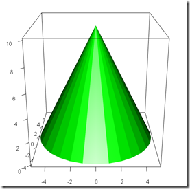
Volume of solids of revolution: the cone

Have you ever wondered where do all those formulas to calculate the volume of solids like a cone, a cylinder, a sphere ecc… come from? In fact they come from a simple formula and from a clever basic idea. Imagine you have a function f

Intuitively you could approximate the volume by dividing your interval into a number n of small intervals of the same size and sum up the volume of the cylinders of radius f(x) and height , then

if we use an infinite number of steps n then our sum becomes an integral:

Now that we have the intuition, we  can go on to the code. I coded an example in R and one in Matlab. The one in Matlab is shorter since it deals with the integration on its own using symbolic computation while in R I decided to code a simple approximation algorithm based on the first formula I posted above, although you could easily calculate the indefinite integral of the function foo and then use it to calculate the exact volume.

Here is the Matlab example, quick, fast and neat:

Note that f(10)=5, thus the radius of our cone is 5. Furthermore, for the sake of simplicity I’ve assumed that the tip is in 0,0. This code outputs:

Here is the R code. Of course you could have made it shorter and more neat but I like coding in R so I made something more out of it. The R program below approximates the volume using the first approach described above.

Finally, you can get a 3D cone as the one at the top of this page just by using the RGL package in R and the demo scripts.

Tag di Technorati: geometry,calculus,R,matlab,programming,volume

How to calculate the length of an arbitrary arc

Have you ever wondered if you could calculate how long is a certain curved path with a “simple formula”? Apparently you can, provided that you are good with integrals (or you can use Wolfram Alpha or Matlab). I am no mathematician and this is by no means a rigorous proof, however I think it surely delivers a first grasp on the underlying concepts.

A first approach could be use a real meter, but then you’d have to deal with the uncertainty that comes with every measurement and bla bla bla… From the deep magic forest of calculus, another approach to lines could become very handy: consider for instance an arbitrary curve S

by considering this as a limit in which the change in S approaches ds and applying the Pythagorean theorem we can write:

Now if your line is in parametric form we just divide by dt squared, if it is in the form f(x) then you can divide by dx squared and then integrate with respect to dx. For this example I am assuming S is in parametric form as such:

Dividing by dt squared yields

and after some manipulations we can integrate and get the length of our line from a to b

Suppose we’d like to calculate the length of the arc of our parametric function from 0 to 10, then assuming my calculations are correct, we’d have to calculate

Now perhaps this is easy to calculate manually, perhaps it isn’t, however it is surely fun to implement in some programming language. Sadly the sympy module in Python for symbolic maths does not work on this integral, it just seems to loop forever, perhaps that’s just my computer or I wrote something wrong. Therefore I used Matlab, which, aside from being somewhat difficult to start on my computer, works perfectly for this kind of tasks. In red is the arc whose length we’d like to calculate.

My simple Matlab script spits out as a solution the number 10.7602 which double checked on Wolfram Alpha seems to be the right solution.

To be fair my code prints out this: log(4*410^(1/2) + 81)/8 + 1640^(1/2)/4 which then computed yields the final result. Here below you can check my code

 

Tag di Technorati: maths,matlab,line,integral,programming