EM Algorithm: Run It and Know When to Trust It

The EM algorithm raises the log-likelihood on every iteration, which every explanation repeats, and the guarantee is only local. I wrote the two steps in numpy, fitted three components to iris petal length, and broke the run twice in ways that still show a climbing number.

What the two steps actually compute

The algorithm fits a model that contains variables you cannot observe, and in a Gaussian mixture those hidden variables are the component each point came from. The two steps take turns guessing them and refitting around the guess.

Step	Input	Output
E	current means, variances and weights	a responsibility between 0 and 1 for every point and component
M	the responsibilities from the E step	refitted means, variances and weights

The likelihood cannot fall because the M step maximises the same quantity the E step built a lower bound around. What the guarantee does not say is where the process stops, and the Stack Overflow thread on the E step is where that belief gets stated as a posterior distribution that guarantees the likelihood increases.

What you need before writing the loop

The loop itself is short, and two decisions inside it change the result more than the loop does.

A numeric library. numpy covers everything here, and scikit-learn ships a version of the same algorithm with the guards already in place.
A single measured column of data, so the components can be checked against something you already know.
A starting point for each component. Random points are the default in hand-written loops and the usual source of a wrong answer.
A stopping rule, either a change in the log-likelihood below a tolerance or a maximum iteration count.
A way to compare runs, because one fit is not evidence about which fit is best.

The starting point and the comparison are the two that decide the outcome, and the runs below show both of them going wrong on numbers small enough to read.

Writing the E step and the M step

Reading the responsibilities as numbers first is what makes the loop worth trusting later. A single pass on five points makes the arithmetic visible before it disappears inside a loop.

import numpy as np

x = np.array([1.0, 1.8, 2.2, 9.9, 10.4])
means = np.array([2.0, 10.0])
variances = np.array([0.5, 0.5])
weights = np.array([0.5, 0.5])


def e_step(values, means, variances, weights):
    density = (
        weights
        * np.exp(-0.5 * (values[:, None] - means) ** 2 / variances)
        / np.sqrt(2 * np.pi * variances)
    )
    return density, density / density.sum(axis=1, keepdims=True)


density, responsibility = e_step(x, means, variances, weights)

print("E step, responsibility of each point for each component")
print("point   comp 1   comp 2")
for value, row in zip(x, responsibility):
    print(f"{value:5.1f}   {row[0]:6.4f}   {row[1]:6.4f}")

print("\nsoft counts :", np.round(responsibility.sum(axis=0), 4))
print("hard counts :", np.round((responsibility > 0.5).sum(axis=0), 4))

mass = responsibility.sum(axis=0)
new_means = (responsibility * x[:, None]).sum(axis=0) / mass
new_variances = (responsibility * (x[:, None] - new_means) ** 2).sum(axis=0) / mass
new_weights = mass / len(x)

print("\nM step")
print("  means    :", np.round(new_means, 4), "was", means)
print("  variances:", np.round(new_variances, 4), "was", variances)
print("  weights  :", np.round(new_weights, 4), "was", weights)

print("\nlog-likelihood before :", round(float(np.log(density.sum(axis=1)).sum()), 4))
density_after, _ = e_step(x, new_means, new_variances, new_weights)
print("log-likelihood after  :", round(float(np.log(density_after.sum(axis=1)).sum()), 4))

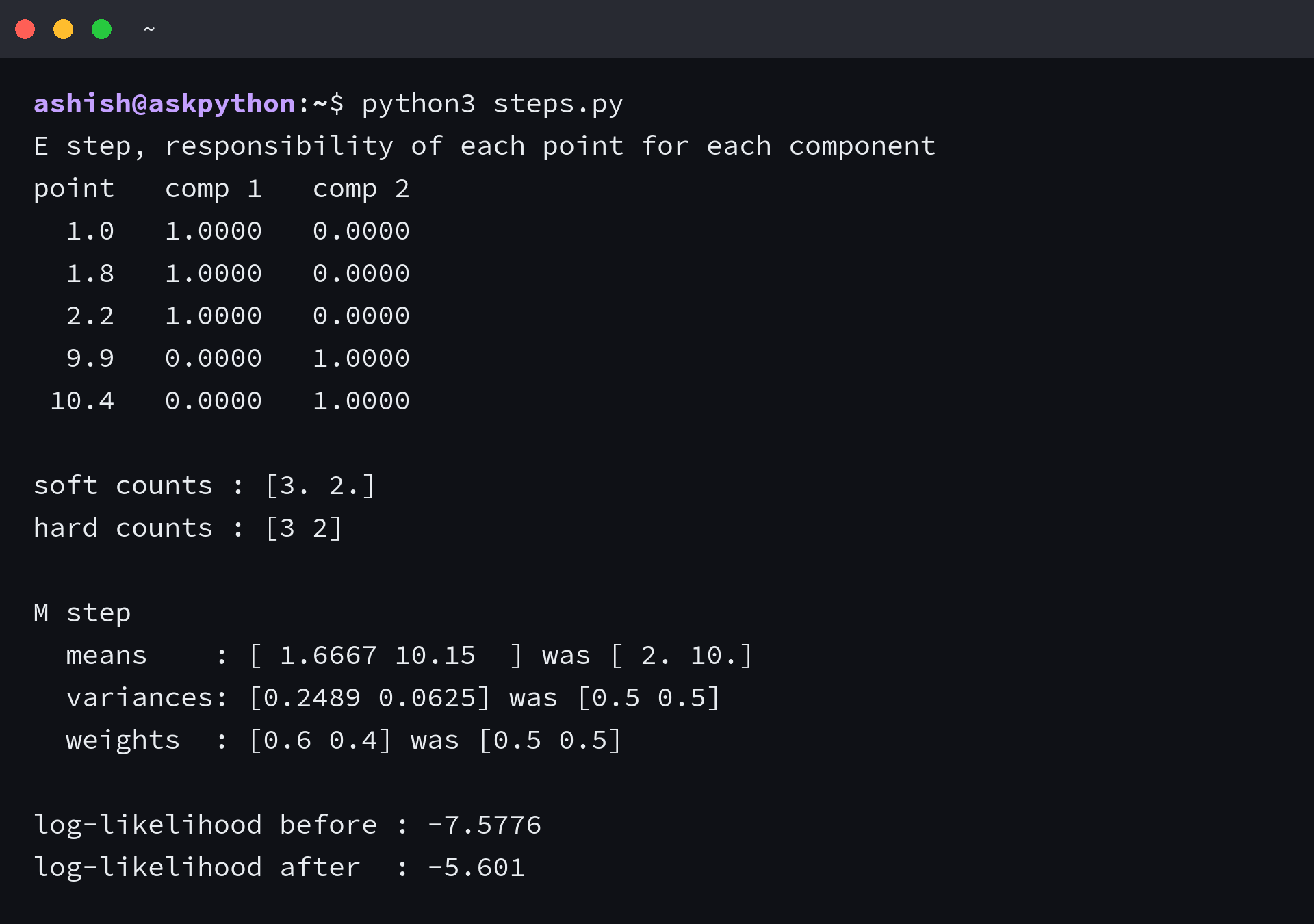
Terminal output from python3 steps.py showing the responsibility of each of five points for two components, the soft and hard counts, the refitted means, variances and weights, and the log-likelihood before and after

I printed the responsibilities as a table, and on these five points they land on 1 and 0 because the two groups sit far apart. A point halfway between the components would split its weight instead, which is the behaviour the soft counts exist to capture.

The M step then pulls both means toward the points they are responsible for, so the lower component moves from 2.0 to 1.6667 and the upper one from 10.0 to 10.15. The log-likelihood rises from -7.5776 to -5.601 across that single pass, which is the whole guarantee in miniature.

Running it on labelled data

Petal length from the iris dataset gives a mixture with a recorded answer, since the species labels ship in the same file.

"""Two-component EM on real data: iris petal length, three components, from scratch."""
import numpy as np
from sklearn.datasets import load_iris

iris = load_iris()
x = iris.data[:, 2]  # petal length in cm


def em_1d(values, k=3, iterations=40, seed=0):
    rng = np.random.default_rng(seed)
    means = rng.choice(values, size=k, replace=False).astype(float)
    variances = np.full(k, values.var())
    weights = np.full(k, 1 / k)
    trace = []

    for _ in range(iterations):
        # E step: how much each point belongs to each component
        density = (
            weights
            * np.exp(-0.5 * (values[:, None] - means) ** 2 / variances)
            / np.sqrt(2 * np.pi * variances)
        )
        responsibility = density / density.sum(axis=1, keepdims=True)

        # M step: refit each component to the points it is responsible for
        mass = responsibility.sum(axis=0)
        means = (responsibility * values[:, None]).sum(axis=0) / mass
        variances = (responsibility * (values[:, None] - means) ** 2).sum(axis=0) / mass
        weights = mass / len(values)

        trace.append(float(np.log(density.sum(axis=1)).sum()))

    return means, variances, weights, trace


means, variances, weights, trace = em_1d(x)

print("iterations run        :", len(trace))
print("log-likelihood first  :", round(trace[0], 4))
print("log-likelihood last   :", round(trace[-1], 4))
print("strictly increasing   :", all(b > a for a, b in zip(trace, trace[1:])))
print("smallest step         :", round(min(b - a for a, b in zip(trace, trace[1:])), 6))
print("\nlearned components")
for mean, var, weight in sorted(zip(means, variances, weights)):
    print(f"  mean {mean:6.3f}   variance {var:6.3f}   weight {weight:5.3f}")

print("\nwhat the species actually look like")
for index, name in enumerate(iris.target_names):
    rows = x[iris.target == index]
    print(f"  {name:12s} mean {rows.mean():6.3f}   share {len(rows) / len(x):5.3f}")

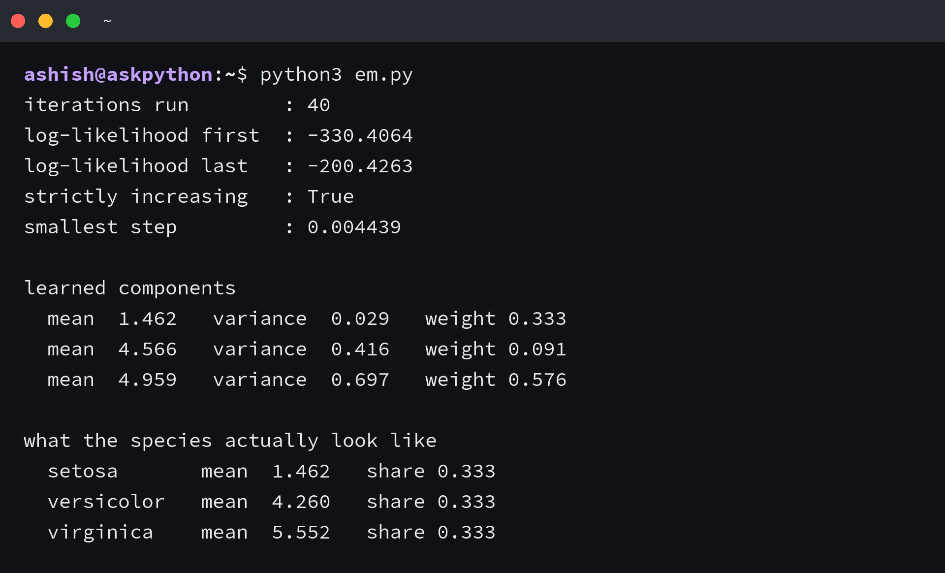
Terminal output from python3 em.py showing a strictly increasing log-likelihood across 40 iterations, the three learned components and the true mean and share of each iris species

I stepped the loop until the trace had climbed from -330.4064 to -200.4263 with no decrease on any pass, which is what the theory promises. The learned components are then read against the species they came from.

Component	Learned mean	Learned variance	Learned weight	Closest species
1	1.462	0.029	0.333	setosa, mean 1.462 and share 0.333
2	4.566	0.416	0.091	versicolor, mean 4.260 and share 0.333
3	4.959	0.697	0.576	virginica, mean 5.552 and share 0.333

The first component found setosa exactly, and the other two divided the remaining hundred flowers between them. Petal length alone does not separate versicolor from virginica, so the mixture is being asked for a distinction the column does not carry, and the climbing number reports nothing about that.

The solution that makes the likelihood infinite

Start one component on a single point with a small variance and the next pass shrinks it further. I set the second mean on a data point with a small variance to see how far the loop would follow it, and the run stops being usable on the following pass.

"""The degenerate solution, and the one line that prevents it."""
import numpy as np

x = np.array([1.0, 1.9, 2.1, 1.8, 9.8, 10.2, 9.9])
FLOOR = 1e-3


def e_step(values, means, variances, weights):
    density = (
        weights
        * np.exp(-0.5 * (values[:, None] - means) ** 2 / variances)
        / np.sqrt(2 * np.pi * variances)
    )
    return density / density.sum(axis=1, keepdims=True), float(np.log(density.sum(axis=1)).sum())


def m_step(values, responsibility, floor=None):
    mass = responsibility.sum(axis=0)
    means = (responsibility * values[:, None]).sum(axis=0) / mass
    variances = (responsibility * (values[:, None] - means) ** 2).sum(axis=0) / mass
    if floor is not None:
        variances = np.maximum(variances, floor)
    return means, variances, mass / len(values)


means = np.array([1.8, 10.2])
variances = np.array([1.0, 0.0001])
weights = np.array([0.5, 0.5])

print("no floor on the variance")
print("step   variance 2   log-likelihood")
for step in range(4):
    responsibility, loglik = e_step(x, means, variances, weights)
    print(f"{step:4d}   {variances[1]:10.6f}   {loglik:14.4f}")
    means, variances, weights = m_step(x, responsibility)

print("\nsame run, floor of", FLOOR)
means = np.array([1.8, 10.2])
variances = np.array([1.0, 0.0001])
weights = np.array([0.5, 0.5])
for step in range(12):
    responsibility, loglik = e_step(x, means, variances, weights)
    if step in (0, 1, 2, 11):
        print(f"{step:4d}   {variances[1]:10.6f}   {loglik:14.4f}")
    means, variances, weights = m_step(x, responsibility, floor=FLOOR)

print("\nfinal means    :", np.round(means, 4))
print("final variances:", np.round(variances, 6))
print("final weights  :", np.round(weights, 4))

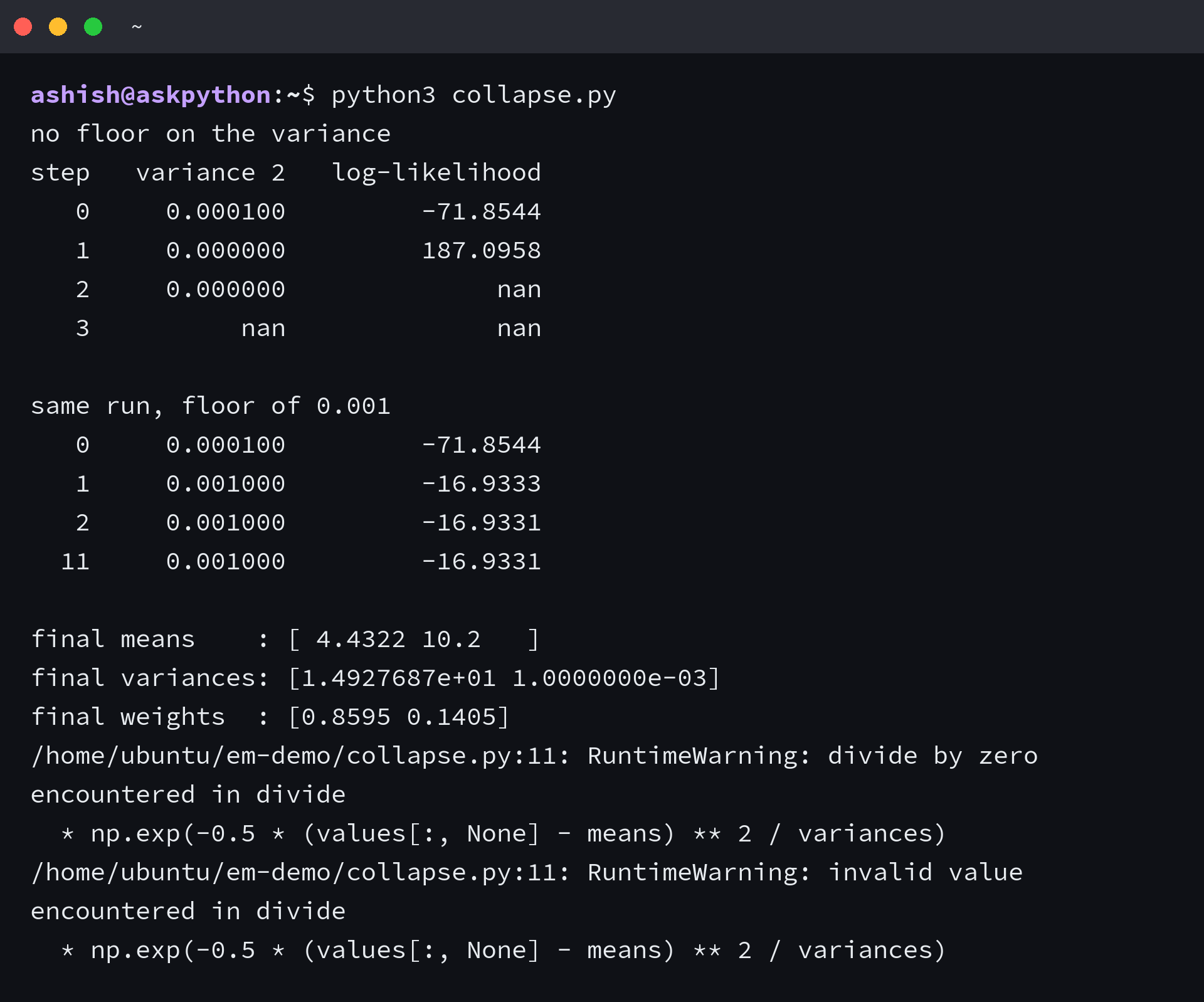
Terminal output from python3 collapse.py showing a component variance falling to zero, the log-likelihood jumping to a large positive number and then nan, followed by the same run held at a variance floor

The variance reached zero and the log-likelihood jumped from -71.8544 to 187.0958, which is not a better fit but a density that is infinite at one point and zero everywhere else. The following iteration returned nan, because dividing by that zero makes every value NaN.

Floors on the variance are the usual answer, and the second half of the run shows what they fix. The number stays finite at -16.9331, and the fit it settles on still pins the collapsed component at 10.2 with a weight of 0.1405 while the other component’s variance inflates to 14.93.

The starting point decides which answer you get

I reproduced the collapse and then ran the same seven points through the library, because the collapse is only an extreme case of a general problem. The likelihood EM climbs belongs to whichever peak it started nearest.

"""What actually fixes the collapse: a starting point that spreads the components out."""
import numpy as np
from sklearn.mixture import GaussianMixture

x = np.array([1.0, 1.9, 2.1, 1.8, 9.8, 10.2, 9.9]).reshape(-1, 1)

model = GaussianMixture(n_components=2, init_params="k-means++", n_init=5, random_state=0)
model.fit(x)

order = np.argsort(model.means_.ravel())
print("k-means++ initialisation")
print("  means    :", np.round(model.means_.ravel()[order], 4))
print("  variances:", np.round(model.covariances_.ravel()[order], 6))
print("  weights  :", np.round(model.weights_[order], 4))
print("  converged:", model.converged_, "in", model.n_iter_, "iterations")

# the same run forced to start from the bad point
bad = GaussianMixture(
    n_components=2,
    init_params="random",
    n_init=1,
    random_state=3,
    reg_covar=1e-6,
)
bad.fit(x)
print("\nrandom initialisation, one restart")
print("  means    :", np.round(bad.means_.ravel(), 4))
print("  variances:", np.round(bad.covariances_.ravel(), 6))
print("  weights  :", np.round(bad.weights_, 4))
print("  converged:", bad.converged_, "in", bad.n_iter_, "iterations")
print("  reg_covar floor in use:", bad.reg_covar)

Terminal output from python3 init.py comparing a k-means++ initialisation that converged in three iterations with a random single-restart initialisation that converged to a different answer in two

Starting point	Means	Variances	Iterations
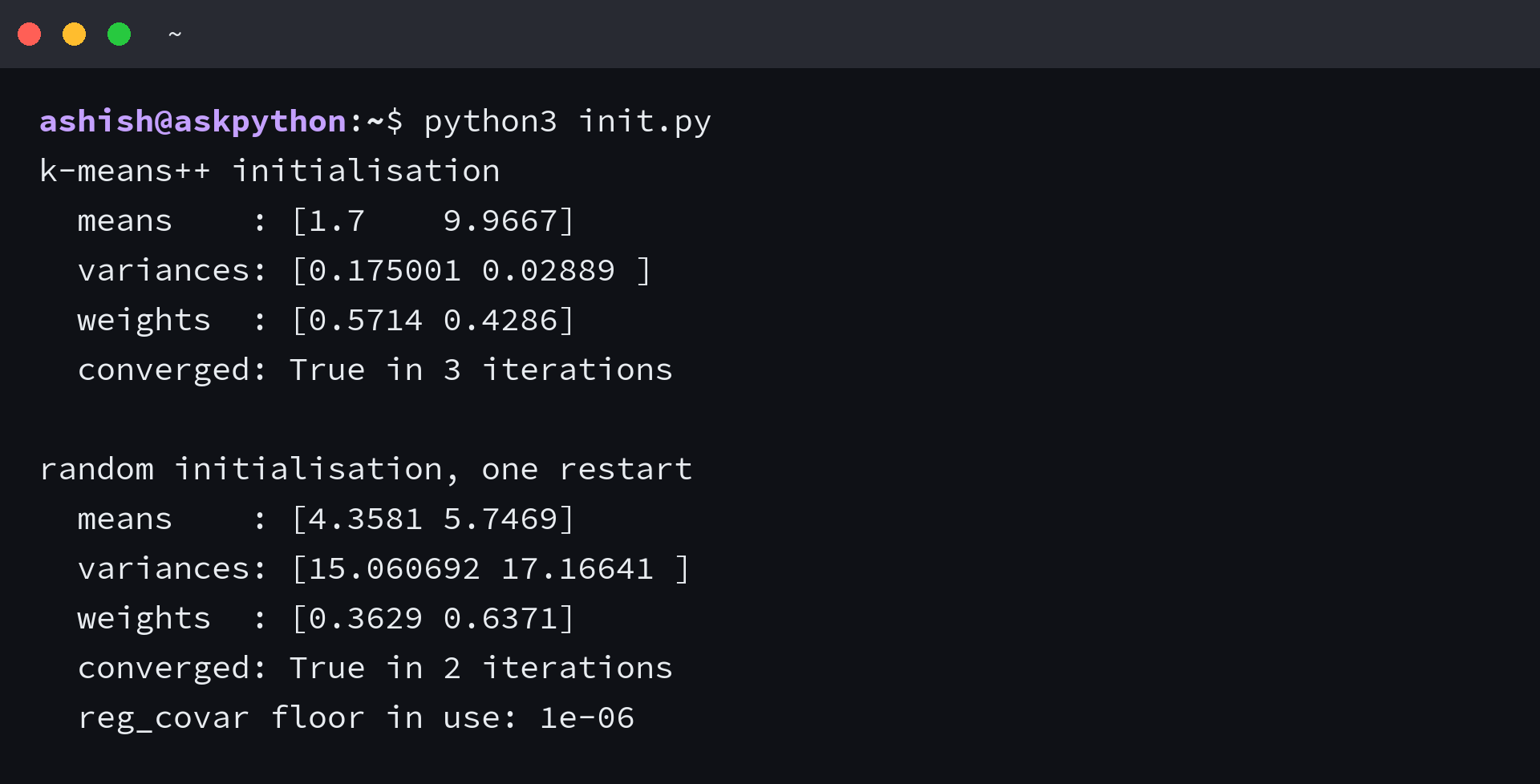
k-means++ over five restarts	1.7 and 9.9667	0.175 and 0.02889	3
random, one restart	4.3581 and 5.7469	15.060692 and 17.16641	2

Both runs report convergence and they are not the same answer. The random start settled into a local optimum where each component covers the whole range, which is worth recognising on sight, because a converged flag in the output means only that the change fell below the tolerance.

The check that separates convergence from noise

I fitted the iris column from five different starting points, because the check rests on two properties and both are cheap to measure. The trace should never fall, and the answer should not move far when the start does.

"""The check to run before trusting a fit: monotone likelihood, and more than one start."""
import numpy as np
from sklearn.datasets import load_iris

x = load_iris().data[:, 2]


def fit(values, k=3, iterations=40, seed=0):
    rng = np.random.default_rng(seed)
    means = rng.choice(values, size=k, replace=False).astype(float)
    variances = np.full(k, values.var())
    weights = np.full(k, 1 / k)
    trace = []
    for _ in range(iterations):
        density = (
            weights
            * np.exp(-0.5 * (values[:, None] - means) ** 2 / variances)
            / np.sqrt(2 * np.pi * variances)
        )
        responsibility = density / density.sum(axis=1, keepdims=True)
        mass = responsibility.sum(axis=0)
        means = (responsibility * values[:, None]).sum(axis=0) / mass
        variances = (responsibility * (values[:, None] - means) ** 2).sum(axis=0) / mass
        weights = mass / len(values)
        trace.append(float(np.log(density.sum(axis=1)).sum()))
    return trace


results = {seed: fit(x, seed=seed) for seed in range(5)}

print("seed   final log-likelihood   largest drop   steps")
for seed, trace in results.items():
    steps = [b - a for a, b in zip(trace, trace[1:])]
    print(f"{seed:4d}   {trace[-1]:20.4f}   {min(steps):12.3e}   {len(trace)}")

best = max(results, key=lambda s: results[s][-1])
print("\nbest seed  :", best, "at", round(results[best][-1], 4))
print("spread     :", round(max(t[-1] for t in results.values()) - min(t[-1] for t in results.values()), 4))
print("tolerance  :", 1e-6, "covers every drop:", all(min(b - a for a, b in zip(t, t[1:])) > -1e-6 for t in results.values()))

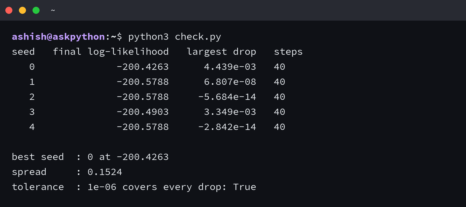
Terminal output from python3 check.py listing the final log-likelihood, the largest drop and the iteration count for five seeds, then the best seed, the spread across seeds and the tolerance result

The largest drop across the five runs is -5.68e-14, which is floating-point noise rather than a decrease, and a tolerance of 1e-6 covers every one of them. The spread is 0.1524, so on this data the start moves the final number without moving it far.

The part worth copying is the comparison rather than the loop. Fit with more starts than you think you need, keep the parameters and not only the score, and check the winner against a grouping you already trust before anything downstream depends on it.

Questions about the EM algorithm

What is the EM algorithm used for?

It fits models that contain variables you cannot measure, which covers Gaussian mixtures, hidden Markov models, missing-data imputation, and topic models. Anywhere a likelihood depends on a hidden label, the two-step structure applies.

Does the EM algorithm always converge?

The log-likelihood never decreases, and the algorithm stops at a local maximum rather than the global one. That is not the same as converging on the right answer, which is why the starting point and a multi-start check both matter.

Why does the log-likelihood become NaN?

One component usually collapsed onto a single point, so its variance reached zero and the density became infinite. The next iteration divides by that zero and every value becomes NaN. A variance floor stops the crash without fixing the bad start.

How many components should I use?

Choose by comparing fits rather than by inspecting the log-likelihood, because it rises with every component you add. The Bayesian information criterion is the common choice, and it penalises the extra parameters.

Is EM the same as k-means?

k-means is the special case where each point belongs to exactly one component and every component has the same fixed variance. EM keeps the responsibilities as probabilities and refits the variances, so it is the softer version of the same loop.

Does scikit-learn use the EM algorithm for Gaussian mixtures?

Yes. GaussianMixture runs the same two steps and adds the guards a hand-written loop lacks, starting from k-means++ by default and adding a small value to every covariance through reg_covar.