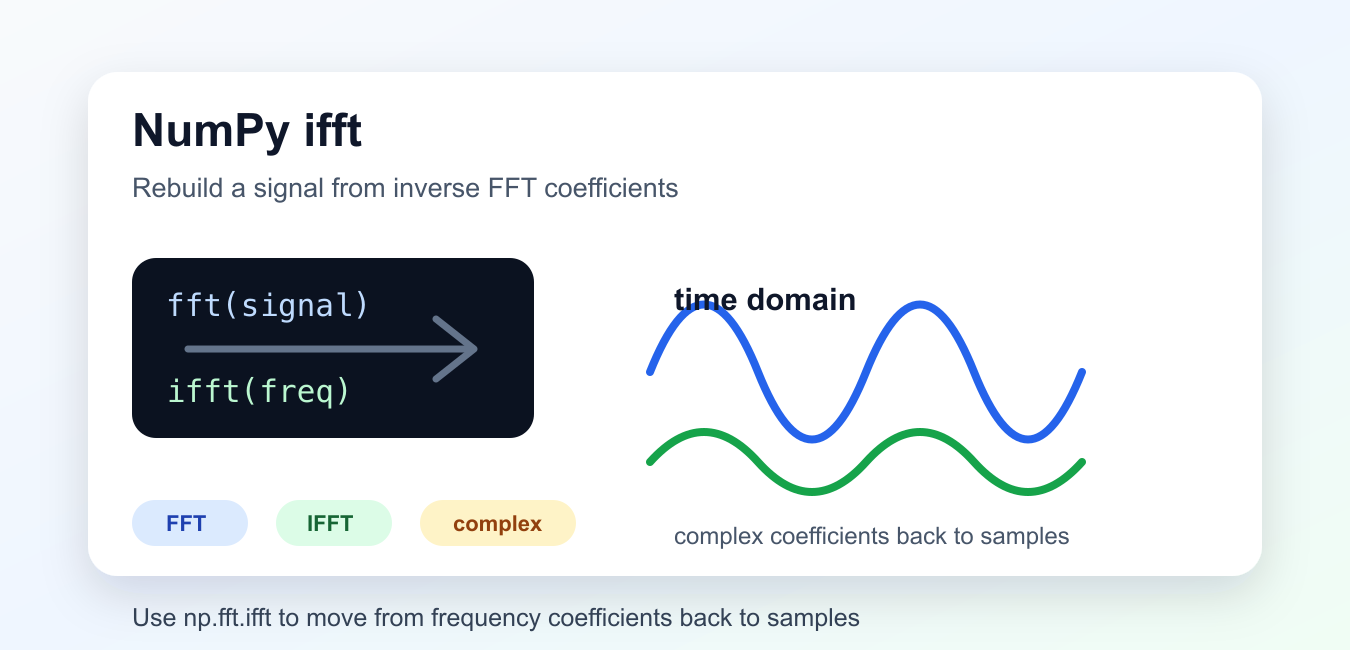
Quick answer: NumPy ifft computes a one-dimensional inverse discrete Fourier transform along a chosen axis. To reconstruct a signal reliably, control the transform length, normalization, complex output, frequency-bin ordering, and numerical tolerance.
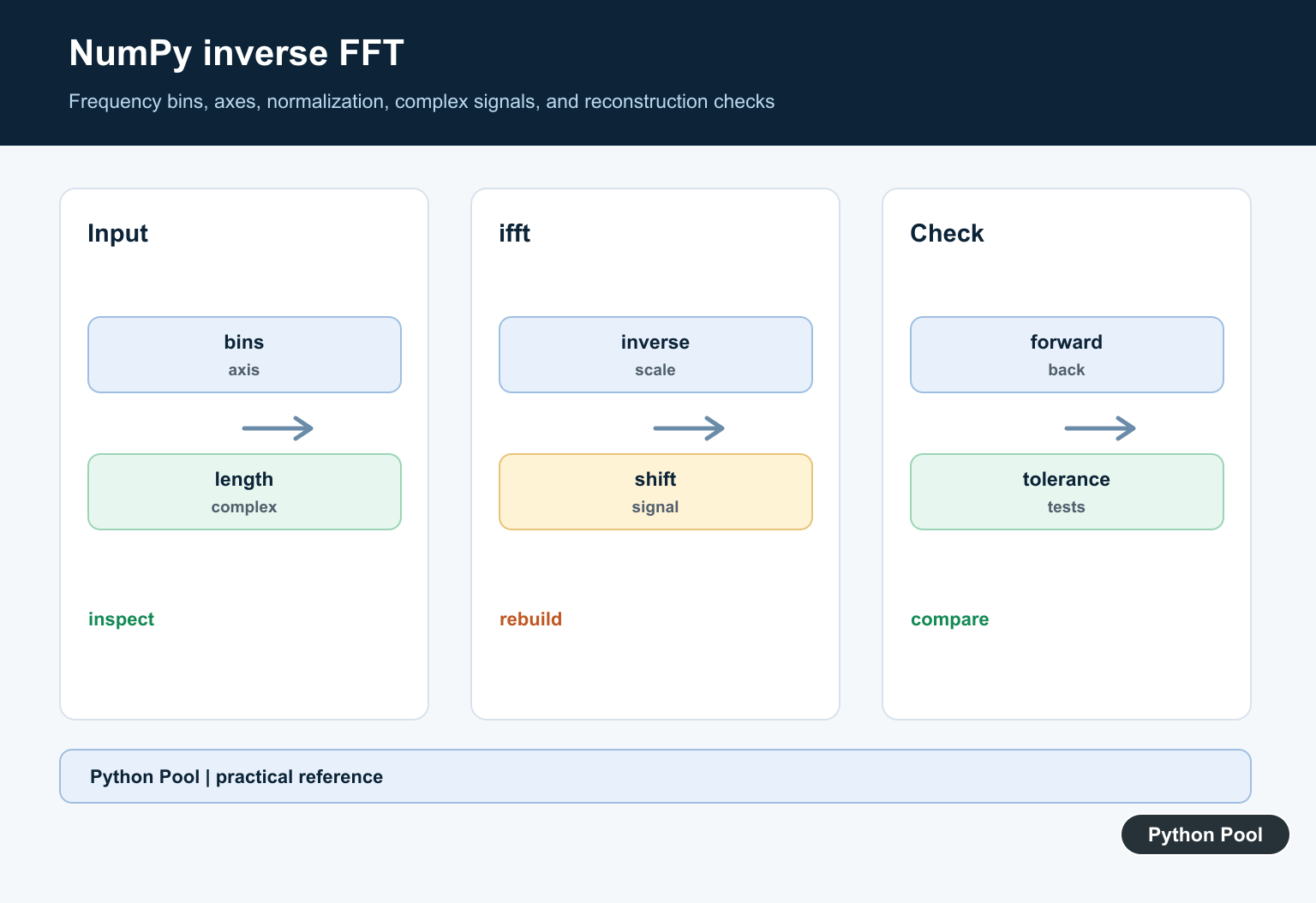
np.fft.ifft() computes the one-dimensional inverse discrete Fourier transform. In practical terms, it turns frequency-domain coefficients back into time-domain samples.
The official NumPy ifft documentation covers the function arguments, while the NumPy FFT routines page explains the transform family. The forward transform is documented at NumPy fft.
Use ifft() after fft() when you need to reconstruct a signal from its complex frequency coefficients. Small floating-point differences are normal, so compare results with a tolerance.
This workflow appears in audio analysis, vibration data, image processing, and numerical experiments. The details can become advanced quickly, but the core API is simple: forward transform with fft(), inverse transform with ifft().
Rebuild A Signal After FFT
The most direct example is a round trip: transform a signal with fft(), then reconstruct it with ifft().
import numpy as np

signal = np.array([1.0, 2.0, 0.0, -1.0])

frequency = np.fft.fft(signal)
rebuilt = np.fft.ifft(frequency)

print(frequency)
print(rebuilt)
print(np.allclose(signal, rebuilt.real))
The inverse result is complex because FFT calculations work in the complex domain. For a real input with ordinary round-trip behavior, the imaginary part should be tiny.
Use np.allclose() instead of exact equality because floating-point transforms can introduce very small numerical differences.
If the original signal is real, use the real part only after confirming that the imaginary part is near zero. That check prevents accidentally hiding a meaningful complex result.
Inspect The Real And Imaginary Parts
After an inverse transform, inspect the real and imaginary parts separately when debugging.
import numpy as np

signal = np.array([0.0, 1.0, 0.0, -1.0])
frequency = np.fft.fft(signal)
rebuilt = np.fft.ifft(frequency)

print(rebuilt.real)
print(rebuilt.imag)
The real part contains the reconstructed samples. The imaginary part often contains values close to zero due to numerical precision.
If the imaginary part is large, check whether the frequency coefficients were changed in a way that should produce a complex output.
Complex output is not automatically an error. It is only suspicious when the math or data source says the reconstructed signal should be real-valued.
Use ifft With A Sine Wave
A generated sine wave makes the round trip easier to see.
import numpy as np

t = np.arange(8)
signal = np.sin(2 * np.pi * t / 8)

frequency = np.fft.fft(signal)
rebuilt = np.fft.ifft(frequency).real

print(np.round(signal, 4))
print(np.round(rebuilt, 4))
The rounded arrays match, showing that the inverse transform rebuilds the original samples from the FFT coefficients.
Rounding is only for display. Keep full precision for calculations that continue after the transform.
For repeatable examples, use a small number of samples and print rounded arrays. For real signal work, keep the full arrays and plot or measure the result instead of relying on printed values.
Control The Output Length
The n argument sets the length of the inverse transform. It can truncate or zero-pad the coefficient array.
import numpy as np

frequency = np.array([6 + 0j, -2 + 2j, -2 + 0j, -2 - 2j])

same_length = np.fft.ifft(frequency)
longer = np.fft.ifft(frequency, n=8)

print(same_length)
print(longer)
Changing n changes the number of output samples. Use it intentionally, especially when matching a target signal length.
If the length is wrong, downstream plots, filters, or comparisons may look shifted or misaligned.
When in doubt, keep n equal to the coefficient length. Change it only when you have a specific padding, truncation, or resampling goal.
Apply A Simple Frequency Filter
A common workflow is to transform a signal, modify selected coefficients, then use ifft() to return to samples.
import numpy as np

signal = np.array([1.0, 1.4, 1.0, -0.2, -1.0, -1.4, -1.0, 0.2])
frequency = np.fft.fft(signal)

filtered_frequency = frequency.copy()
filtered_frequency[3:-2] = 0

filtered_signal = np.fft.ifft(filtered_frequency).real

print(np.round(filtered_signal, 3))
This is a simplified demonstration, not a complete signal-processing filter design. It shows the pattern of editing coefficients before reconstruction.
In real analysis, choose coefficient ranges based on sampling rate, desired cutoff, and the properties of the signal.
Also remember that FFT coefficient order has a specific layout. For serious filtering, study the frequency bins before deciding which coefficients to keep or remove.
Use ifft Along An Axis
For multidimensional arrays, the axis argument chooses the direction of the inverse transform.
import numpy as np

signals = np.array([
    [1.0, 0.0, -1.0, 0.0],
    [0.0, 1.0, 0.0, -1.0],
])

frequency = np.fft.fft(signals, axis=1)
rebuilt = np.fft.ifft(frequency, axis=1).real

print(np.round(rebuilt, 3))
Here each row is treated as its own signal because axis=1 transforms across columns.
Always choose the axis deliberately. Transforming down columns instead of across rows changes the meaning of the output.
A useful habit is to print the input and output shapes around transform code. Shape checks catch many axis mistakes before the numeric result is interpreted.
Common ifft Mistakes
Do not expect exact equality after an FFT and inverse FFT round trip. Use np.allclose() or rounded display output for checks.
Do not discard the imaginary part blindly when the input coefficients are not expected to represent a real signal. A complex result may be meaningful.
Do not change n or axis without checking the resulting shape. Shape mismatches can break later code even when the transform itself succeeds.
The practical default is to compute coefficients with np.fft.fft(), modify or inspect them, then use np.fft.ifft() and compare the reconstructed samples with a tolerance.
Match The Transform Pair
Use fft and ifft with the same length, axis, and normalization policy. Padding or truncation changes the sample grid, so treat n as part of the signal contract rather than an incidental argument.
Choose The Correct Axis
For a multidimensional array, the default axis is the last one. Inspect shapes and use axis or ifftn explicitly when frequency bins live elsewhere or multiple dimensions are transformed.
Understand Complex Results
An inverse transform generally returns complex values. Tiny imaginary parts can be roundoff for an expected real signal, but discard them only after checking the model and conjugate symmetry.
Control Normalization
NumPy’s default scaling puts the inverse factor in the inverse transform. Use the documented norm option when matching another FFT implementation or a physical signal-processing convention.
Inspect Frequency Ordering
The zero-frequency term and positive and negative frequencies have defined positions. Use fftshift only for display or a deliberately shifted representation, not as an unexplained preprocessing step.
Verify Reconstruction
Transform known time-domain data forward and back, compare with an absolute and relative tolerance, test real and complex inputs, non-power-of-two lengths, axes, empty or short arrays, and malformed shapes.
Use the official NumPy ifft documentation for axes, length, and normalization. Related Python Pool references include NumPy arrays and tests.
For related numerical workflows, compare NumPy array axes, reconstruction tests, and sample sequences before applying an inverse FFT.
Frequently Asked Questions
What does NumPy ifft do?
ifft computes the one-dimensional inverse discrete Fourier transform along an axis, converting frequency-domain samples into time-domain samples.
Why does ifft return complex values?
The transform is generally complex; a real signal can produce tiny imaginary roundoff terms that should be handled with an explicit real-value policy after validation.
How do I choose the ifft axis?
Choose the axis that contains the frequency bins and verify the array shape before transforming multi-dimensional data; use ifftn or axes for multiple dimensions.
How can I verify an inverse FFT?
Transform known data forward and back, compare within numerical tolerances, check scaling and length, and inspect conjugate symmetry when a real signal is expected.
