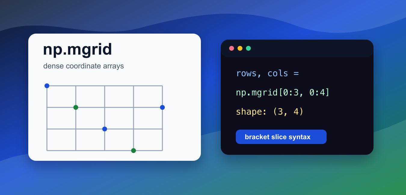
Quick answer: np.mgrid is an indexing object that creates dense coordinate arrays from slice notation. A normal integer step behaves like arange and excludes the stop value; a complex step such as 5j requests a number of evenly spaced points including the endpoint. Because mgrid materializes full coordinate planes, compare ogrid or sparse meshgrid when grid size makes memory important.
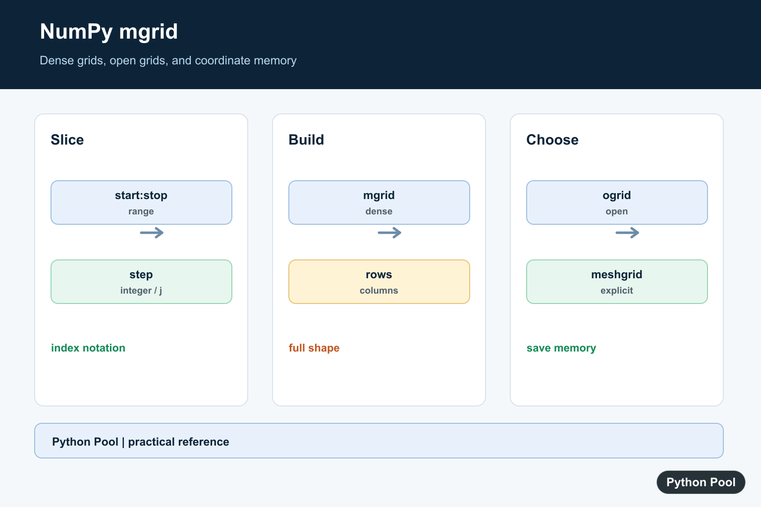
numpy.mgrid creates dense coordinate arrays from slice syntax. It is commonly described as mgrid(), but you use square brackets such as np.mgrid[0:3, 0:4] rather than a normal function call.
The official NumPy documentation covers numpy.mgrid, numpy.ogrid, and numpy.meshgrid().
Use mgrid when you want full row and column coordinate arrays. The result is dense, which means each output has the full grid shape. This is convenient for calculations, but it can use more memory than open-grid forms.
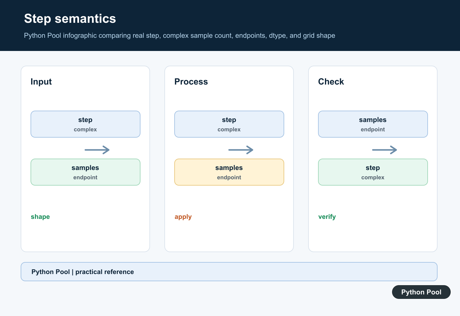
The slice syntax follows familiar start, stop, and step rules. A normal integer step behaves like arange() and stops before the endpoint. A complex step such as 5j asks NumPy for five evenly spaced points, including the endpoint.
For image-like arrays, matrix coordinates, distance maps, and surface calculations, mgrid can make the coordinate setup compact and readable.
For very large grids, compare it with ogrid. ogrid returns open coordinate arrays that broadcast together without storing every full coordinate plane.
Another common choice is meshgrid(), which builds coordinate arrays from existing one-dimensional coordinate inputs. Use mgrid when the coordinate ranges are naturally expressed as slices. Use meshgrid() when you already have coordinate arrays from another calculation.
Be deliberate about axis order. In many array workflows, the first coordinate corresponds to rows and the second coordinate corresponds to columns. Naming the outputs as rows and cols, or y and x, prevents confusion later.
Create A 1D Grid
A single slice creates one coordinate array.
import numpy as np

grid = np.mgrid[0:5]

print(grid)
This returns values from 0 through 4.
The endpoint is excluded because the slice uses a normal integer step.
This behavior is similar to np.arange(0, 5).
A one-dimensional grid is useful for checking syntax before moving to two axes.
It is also useful for quick index ranges where you want an array result immediately. For larger coordinate systems, the same slice idea extends cleanly to multiple axes. mgrid creates dense coordinate arrays, while NumPy ix_ Guide for Open Mesh Indexing creates an open mesh for selecting combinations of row and column indexes.
Create A 2D Dense Grid
Pass two slices to create row and column coordinate arrays.
import numpy as np

rows, cols = np.mgrid[0:3, 0:4]

print(rows)
print(cols)
print(rows.shape, cols.shape)
Both outputs have shape (3, 4).
The first output stores row coordinates across each column.
The second output stores column coordinates across each row.
Because both arrays have the same shape, you can combine them directly in element-wise formulas.
This is the main reason to choose dense grids: every coordinate array lines up cell by cell. That makes the later formula look almost the same as the mathematical expression you are trying to implement.
Use Complex Step Counts
A complex step such as 5j means the number of points to generate.
import numpy as np

x, y = np.mgrid[0:1:5j, 0:1:3j]

print(x)
print(y)
Here, the first axis has five points and the second axis has three points.
With complex step counts, the endpoint is included.
This is useful when you need a fixed number of samples across a numeric interval.
Use this form for coordinate samples where endpoint inclusion matters.
The complex step notation is easy to miss because the letter j usually marks complex numbers in Python. In this slice position, NumPy uses it as a compact way to request a count of evenly spaced samples.
Compare mgrid And ogrid
mgrid creates dense arrays. ogrid creates open arrays that broadcast together.
import numpy as np

dense_rows, dense_cols = np.mgrid[0:3, 0:4]
open_rows, open_cols = np.ogrid[0:3, 0:4]

print(dense_rows.shape, dense_cols.shape)
print(open_rows.shape, open_cols.shape)
The dense arrays both have the full grid shape.
The open arrays have shapes that are smaller but still broadcast across the grid.
Use mgrid when full coordinate arrays make later code clearer.
Use ogrid when memory use matters and broadcasting is enough.
For small examples, both approaches are easy to inspect. For high-resolution surfaces, dense arrays can become large quickly, so checking shapes before a full calculation is a good habit.
Calculate Distances On A Grid
Coordinate arrays are often used in formulas.
import numpy as np

y, x = np.mgrid[-2:3, -2:3]

distance = np.sqrt(x**2 + y**2)

print(distance)
This calculates each cell distance from the center point.
The row and column coordinates are combined element by element.
The same pattern works for masks, kernels, surfaces, and spatial calculations.
Use clear names for axes so row-column order does not become confusing.
The same approach can create circular masks, radial weights, or simple coordinate-based filters. Since the coordinate arrays are ordinary NumPy arrays, every usual element-wise operation is available.
Build Coordinate Pairs
You can flatten coordinate arrays and stack them into coordinate pairs.
import numpy as np

rows, cols = np.mgrid[0:2, 0:3]

pairs = np.stack((rows.ravel(), cols.ravel()), axis=-1)

print(pairs)
This produces row-column pairs for every grid cell.
The pattern is useful when another tool expects coordinates as one pair per row.
In short, use np.mgrid[...] for dense coordinate arrays, use complex steps for fixed inclusive samples, and consider ogrid when broadcasting can avoid storing full grids.
Read The Slice Shape
For two dimensions, mgrid returns one stacked array whose first axis identifies the coordinate dimension and whose remaining axes are the grid rows and columns. Naming the result carefully prevents confusing row coordinates with column coordinates.
import numpy as np

coords = np.mgrid[0:3, 10:14]
rows = coords[0]
cols = coords[1]
print(coords.shape)
print(rows)
print(cols)
Use A Complex Step For Exact Counts
The complex-step form is useful when the number of samples matters more than the step size. The imaginary part is not a complex coordinate here; its integer magnitude requests the number of points, including the stop endpoint.
import numpy as np

points = np.mgrid[-1:1:5j]
print(points)
print(len(points))
print(points[0], points[-1])
Compare Dense And Open Grids
mgrid stores every coordinate plane at full size. ogrid stores one non-singleton dimension per coordinate, and later NumPy operations broadcast those arrays when a full result is actually needed. This can reduce intermediate memory for separable calculations.
import numpy as np

full = np.mgrid[0:1000, 0:2000]
open_grid = np.ogrid[0:1000, 0:2000]
print(full.shape)
print(open_grid[0].shape, open_grid[1].shape)

distance = open_grid[0] ** 2 + open_grid[1] ** 2
print(distance.shape)
Use meshgrid When Inputs Already Exist
meshgrid is often clearer when x and y vectors come from another calculation or when indexing=’ij’ versus indexing=’xy’ must be explicit. sparse=True provides open-style arrays without using mgrid slice notation.
import numpy as np

x = np.linspace(-1, 1, 4)
y = np.linspace(0, 2, 3)
X, Y = np.meshgrid(x, y, indexing="ij", sparse=True)
field = X ** 2 + Y ** 2
print(X.shape, Y.shape)
print(field.shape)
NumPy documents mgrid as a dense multi-dimensional mesh-grid and explains its integer and complex slice steps. The ogrid reference covers open grids, while meshgrid documents indexing and sparse output. Related references include ogrid, arange, and reshaping grids.
For related coordinate-grid choices, compare ogrid, arange(), and reshaping arrays before materializing a large dense grid.
Frequently Asked Questions
What is NumPy mgrid?
np.mgrid is an indexing object that creates dense multi-dimensional mesh grids from slice notation, with each coordinate array sharing the full grid shape.
Does mgrid include the stop value?
A normal integer step excludes the stop value, while a complex step such as 5j requests a number of evenly spaced points including the endpoint.
What is the difference between mgrid and ogrid?
mgrid returns dense coordinate arrays, while ogrid returns open arrays that broadcast together and usually use less memory.
When should I use meshgrid instead of mgrid?
Use meshgrid when you already have one-dimensional coordinate vectors or need explicit indexing and sparse options; use mgrid when slice notation is the clearest input.
