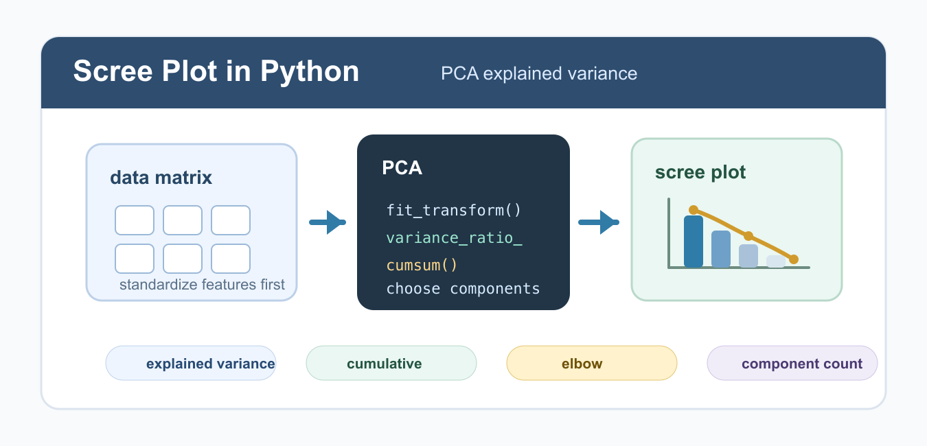
Quick answer: A scree plot displays the variance explained by each PCA component. Build it from sklearn PCA’s explained_variance_ratio_, inspect cumulative variance, and validate the chosen number of components against the downstream task instead of treating an elbow as an automatic answer.
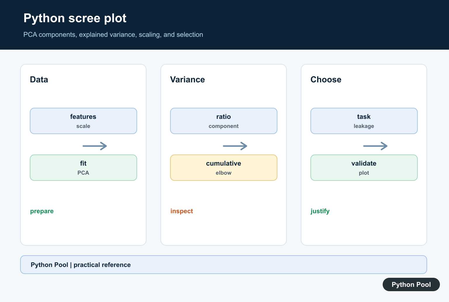
A scree plot in Python helps you choose how many principal components to keep after PCA. It plots the variance explained by each component, usually with component number on the x-axis and explained variance ratio on the y-axis. The point where the curve starts flattening is often called the elbow, and it gives a practical starting point for dimensionality reduction.
In scikit-learn, PCA exposes explained_variance_ratio_ after fitting. That array is exactly what you need for a scree plot. A cumulative variance line is also useful because it shows how many components are required to keep a target amount of information, such as 90% or 95% of total variance.
The chart should guide a decision, not make it automatically. A small elbow means extra components add little variance, but the best count still depends on your model, noise level, storage limits, and whether the reduced features remain interpretable.
Fit PCA and Get Explained Variance
Start by scaling the features, then fit PCA. scikit-learn PCA centers the input data, but it does not scale each feature for you. If your columns use different units or ranges, StandardScaler keeps high-magnitude columns from dominating the first principal components.
import numpy as np
from sklearn.datasets import load_wine
from sklearn.decomposition import PCA
from sklearn.preprocessing import StandardScaler

X, y = load_wine(return_X_y=True)
X_scaled = StandardScaler().fit_transform(X)

pca = PCA()
X_pca = pca.fit_transform(X_scaled)
explained_variance = pca.explained_variance_ratio_

print(explained_variance[:5])
Leaving n_components unset keeps all possible components, which is best when building the first diagnostic plot. After reviewing the plot, you can refit PCA with a smaller component count.
Create a Basic Scree Plot
The simplest scree plot is a line chart with one point per component. Add markers so the component positions remain clear. If you want more Matplotlib marker options, see the guide to Matplotlib markers.
import matplotlib.pyplot as plt
import numpy as np

components = np.arange(1, len(explained_variance) + 1)

plt.plot(components, explained_variance, marker="o")
plt.xlabel("Principal component")
plt.ylabel("Explained variance ratio")
plt.title("Scree plot")
plt.xticks(components)
plt.grid(True, alpha=0.3)
plt.show()
The first few points usually explain the largest share of variance. Later points often contribute less, which is why the plot slopes downward and then starts to flatten.
Add Cumulative Explained Variance
A scree plot is easier to use when it also shows cumulative variance. Bars show each individual component, while a line shows the running total. This makes it clear whether the elbow also satisfies a variance-retention target.
import matplotlib.pyplot as plt
import numpy as np

components = np.arange(1, len(explained_variance) + 1)
cumulative_variance = np.cumsum(explained_variance)

fig, ax = plt.subplots()
ax.bar(components, explained_variance, alpha=0.7, label="Individual")
ax.plot(components, cumulative_variance, marker="o", color="red", label="Cumulative")
ax.set_xlabel("Principal component")
ax.set_ylabel("Explained variance ratio")
ax.legend()
plt.show()
Bars are useful when the exact contribution of each component matters. The PythonPool guide to Matplotlib bar charts covers related formatting options for labels, grouped bars, and stacked bars.
Choose Components by Variance Threshold
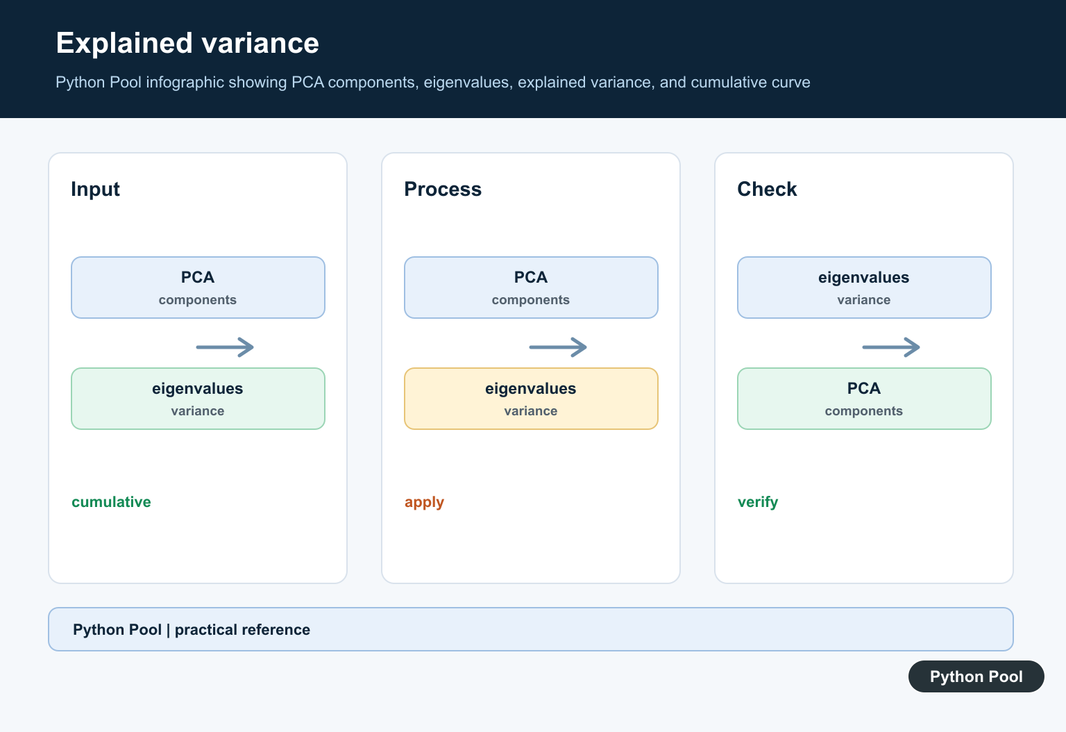
For a reproducible rule, choose the smallest number of components whose cumulative explained variance reaches a target. This does not replace model validation, but it gives you a defensible PCA starting point.
import numpy as np

cumulative_variance = np.cumsum(explained_variance)
threshold = 0.90
n_components = np.argmax(cumulative_variance >= threshold) + 1

print(f"Keep {n_components} components")
print(f"Cumulative variance: {cumulative_variance[n_components - 1]:.2%}")
A 90% threshold is common for exploration, while stricter workflows may use 95% or compare several values. For noisy data, keeping too many low-variance components can preserve noise rather than useful signal.
Build a Reusable Scree Plot Function
If you create scree plots often, wrap the process in a function. The function below scales the data, fits PCA, plots individual and cumulative explained variance, and returns the fitted PCA object for later inspection.
import matplotlib.pyplot as plt
import numpy as np
from sklearn.decomposition import PCA
from sklearn.preprocessing import StandardScaler

def make_scree_plot(X):
    X_scaled = StandardScaler().fit_transform(X)
    pca = PCA().fit(X_scaled)
    ratios = pca.explained_variance_ratio_
    components = np.arange(1, len(ratios) + 1)

    plt.plot(components, ratios, marker="o", label="Individual")
    plt.plot(components, np.cumsum(ratios), marker="s", label="Cumulative")
    plt.xlabel("Principal component")
    plt.ylabel("Explained variance ratio")
    plt.legend()
    plt.show()
    return pca
Returning the fitted PCA object lets you inspect components_, explained_variance_, and transformed shapes without recomputing PCA.
Refit PCA With the Selected Count
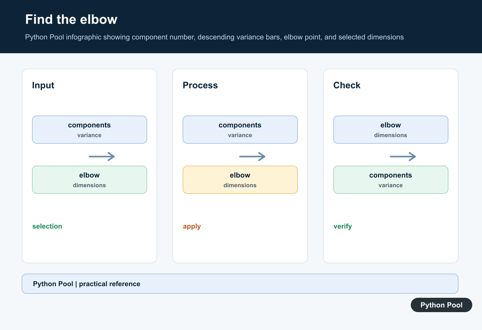
After choosing a component count, refit PCA with n_components. The transformed matrix will have the same number of rows as the original data, but fewer columns. That reduced matrix can then feed a model, clustering step, or visualization.
from sklearn.decomposition import PCA

selected_components = n_components
pca_final = PCA(n_components=selected_components)
X_reduced = pca_final.fit_transform(X_scaled)

print(X.shape)
print(X_reduced.shape)
Use the scree plot as a diagnostic, not as the only decision rule. Downstream accuracy, reconstruction error, clustering quality, or domain constraints may point to a different number of components.
Common Mistakes
The most common mistake is skipping feature scaling before PCA. Another is choosing the elbow by eye without checking cumulative variance. A third is assuming every low-variance component is useless; in some datasets, a low-variance direction can still be meaningful for a specific target.
If your data is time-based, first check whether PCA is the right tool. For lagged relationships, the guide to autocorrelation in Python may be more relevant. For quick summaries of explained variance values, the guide to averages in Python covers basic aggregation patterns.
References
- scikit-learn PCA documentation
- scikit-learn PCA user guide
- scikit-learn StandardScaler documentation
- Matplotlib plot documentation
- NumPy cumsum documentation
Prepare Features Correctly
Align rows, handle missing values, and scale features when units or variances differ. PCA is sensitive to scale, so fitting it directly on mixed-unit features can make the scree plot answer a different question than intended.
Fit PCA And Read Variance
After fitting PCA, explained_variance_ratio_ contains the fraction attributed to each component. Plot component numbers starting at one so the axis matches how results are communicated to readers.
Add Cumulative Variance
A second line or companion plot can show cumulative explained variance. It helps quantify how many components are needed for a chosen retention target, but that target should be justified by the application.
Interpret The Elbow Carefully
The elbow is a visual heuristic, not a theorem. If the curve has no clear bend, compare candidate dimensions with reconstruction error, downstream validation, speed, storage, and interpretability.
Avoid Leakage
Fit scaling and PCA on training data inside the evaluation pipeline, then transform validation or test data with the fitted objects. Fitting on all data can make component selection and model scores optimistic.
Test The Plot Inputs
Use a small matrix with known variance structure, assert component and ratio shapes, confirm ratios sum appropriately, and inspect the saved figure for labels, ticks, and a readable legend.
The official scikit-learn PCA reference documents explained variance. Related Python Pool references include arrays and tests.
For related dimensionality reduction, compare feature arrays, validation tests, and error metrics when choosing components.
Frequently Asked Questions
What does a scree plot show?
It plots the variance explained by each PCA component, helping identify where additional components provide diminishing returns.
How do I make a scree plot in Python?
Fit sklearn PCA, read explained_variance_ratio_, and plot the component numbers against those ratios with Matplotlib.
How many PCA components should I keep?
Use explained variance and cumulative variance as evidence, then validate the chosen dimension against the downstream task rather than relying on an elbow alone.
Should PCA be fit before or after scaling?
For features with different units, scaling before PCA is commonly important because unscaled variance can let a large-unit feature dominate the components.
