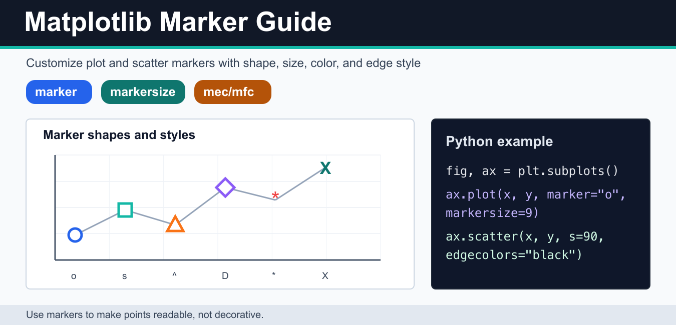
Matplotlib Markers: Style plot() and scatter() Points

Matplotlib markers make individual observations easier to read in a line chart, scatter plot, or diagnostic figure. A marker is the symbol drawn at each data point, such as a circle, square, triangle, or plus sign. The most reliable way to control one is to separate the marker shape from its size, face color, edge color, and transparency. That keeps a plot understandable when the data or the display size changes.

Contents

Quick answer

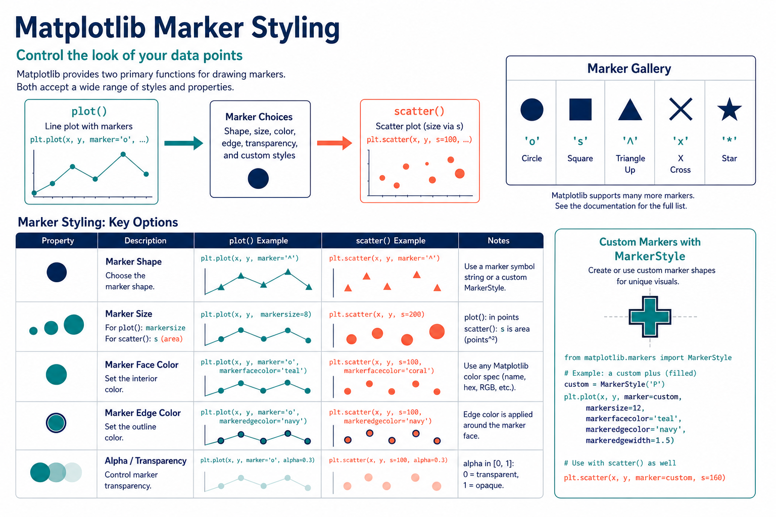
Use marker with plot() or scatter(). For a line plot, set markersize or its short form ms. For a scatter plot, use s, which represents marker area in points squared, so it does not have the same numeric meaning as markersize. Use markerfacecolor and markeredgecolor with plot(), or facecolors and edgecolors with scatter().

The official Matplotlib marker reference lists built-in marker codes and the MarkerStyle class. The examples below use the object-oriented Axes API so the same ideas work in figures with multiple plots.

Matplotlib marker styling guide comparing plot and scatter marker shape size face edge color and alpha — Choose the marker shape, size, face, edge, and transparency separately so plot and scatter stay predictable.

Choose a marker with plot()

The plot() function can draw a line, markers, or both. A format string such as "o-" is compact, but named keyword arguments are easier to review when a figure has several visual rules. Set linestyle="-" for a connecting line and choose a marker separately.

import matplotlib.pyplot as plt

x = [1, 2, 3, 4]
y = [2, 5, 3, 7]

fig, ax = plt.subplots()
ax.plot(
    x,
    y,
    marker="o",
    markersize=8,
    linestyle="-",
    linewidth=1.5,
    markerfacecolor="white",
    markeredgecolor="tab:blue",
    color="tab:blue",
)
ax.set_xlabel("sample")
ax.set_ylabel("value")
plt.show()

For a marker-only line plot, use linestyle="None". This is useful when the x values are ordered but a connecting segment would suggest a relationship that does not exist. Common marker codes include "o" for a circle, "s" for a square, "^" for an upward triangle, "v" for a downward triangle, "D" for a diamond, and "x" for an x.

Python Pool infographic showing Matplotlib x y data, markers, lines, scatter points, and a plot — Plot points: Matplotlib x y data, markers, lines, scatter points, and a plot.

Set marker size and colors

With plot(), markersize controls the marker diameter in points. The edge and face can be styled independently. A white or transparent face with a strong edge is often useful when several lines overlap, while a filled face is easier to see in a dense series.

import matplotlib.pyplot as plt

fig, ax = plt.subplots()
ax.plot(
    [0, 1, 2, 3],
    [4, 2, 5, 3],
    marker="D",
    markersize=9,
    markerfacecolor="gold",
    markeredgecolor="black",
    markeredgewidth=1.2,
    color="black",
    linestyle="--",
)
ax.set_title("Styled diamond markers")
plt.show()

Marker size is a display choice, not a data value. Start with a moderate size and inspect the figure at the size readers will actually see. Oversized symbols can hide neighboring points, while tiny symbols disappear after an image is scaled down.

Python Pool infographic comparing circle, square, triangle, custom path, size, and edge color — Marker styles: Circle, square, triangle, custom path, size, and edge color.

Use scatter() for independent point styling

scatter() is designed for point clouds and can map a numeric column to color, size, or both. Its s argument is marker area in points squared. This means increasing s from 25 to 100 makes the area four times larger, not the diameter four times larger.

import matplotlib.pyplot as plt

x = [1, 2, 3, 4, 5]
y = [4, 2, 5, 3, 6]
sizes = [25, 50, 90, 140, 220]

fig, ax = plt.subplots()
points = ax.scatter(
    x,
    y,
    s=sizes,
    c=y,
    cmap="viridis",
    marker="o",
    alpha=0.8,
    edgecolors="black",
    linewidths=0.7,
)
fig.colorbar(points, ax=ax, label="value")
plt.show()

When every point should look the same, pass one scalar size and one color. When colors represent measurements, label the colorbar and choose a scale that matches the meaning of the data. Do not use size and color simultaneously for unrelated variables unless the legend explains both encodings.

Understand plot markers versus scatter markers

The same marker code can be used by both functions, but their sizing and styling APIs are intentionally different. plot() uses line-oriented properties such as markersize, markerfacecolor, and markeredgecolor. scatter() uses collection properties such as s, facecolors, and edgecolors. Passing a property from one API to the other can produce an error or have no effect.

import matplotlib.pyplot as plt

fig, axes = plt.subplots(1, 2, figsize=(8, 3))
axes[0].plot(
    [1, 2, 3],
    [2, 4, 3],
    marker="o",
    markersize=10,
    markerfacecolor="none",
    markeredgecolor="tab:blue",
)
axes[0].set_title("plot")
axes[1].scatter(
    [1, 2, 3],
    [2, 4, 3],
    s=100,
    facecolors="none",
    edgecolors="tab:orange",
)
axes[1].set_title("scatter")
plt.tight_layout()
plt.show()

The panels above are visually similar but not numerically equivalent. If you are migrating code from one function to the other, retune the size after checking the rendered result. The marker edge can also appear thicker in a dense point collection because many edges are drawn close together.

Python Pool infographic mapping marker size, color, alpha, face, edge, and legend meaning — Encode data: Marker size, color, alpha, face, edge, and legend meaning.

Use alpha without losing contrast

The alpha value controls opacity from zero to one. Lower opacity can reveal dense regions in a scatter plot, but it also weakens the edge and the perceived color. A dark edge with a partially transparent face is often more legible than making the entire marker transparent.

import numpy as np
import matplotlib.pyplot as plt

rng = np.random.default_rng(7)
x = rng.normal(size=400)
y = 0.6 * x + rng.normal(size=400)

fig, ax = plt.subplots()
ax.scatter(
    x,
    y,
    s=32,
    marker="o",
    facecolors="tab:blue",
    edgecolors="white",
    linewidths=0.35,
    alpha=0.55,
)
ax.set_xlabel("x")
ax.set_ylabel("y")
plt.show()

Do not rely on alpha alone to distinguish categories. Add a legend, a shape difference, or a direct label when the category matters. This improves grayscale printing and helps readers with color-vision differences.

Python Pool infographic testing dense points, clipping, legends, savefig, and accessibility — Marker checks: Dense points, clipping, legends, savefig, and accessibility.

Use a custom MarkerStyle

Built-in markers cover most charts. For a reusable custom symbol, create a MarkerStyle object or use a small path. A custom marker should be simple enough to remain recognizable at the final output size. The marker reference documents supported tuple forms and transformations.

import matplotlib.pyplot as plt
from matplotlib.markers import MarkerStyle

marker = MarkerStyle((5, 0, 30))

fig, ax = plt.subplots()
ax.plot(
    [1, 2, 3],
    [3, 5, 4],
    marker=marker,
    markersize=12,
    linestyle="None",
    color="tab:green",
)
ax.set_xlim(0.5, 3.5)
plt.show()

Test a custom marker alongside the built-in symbols it must be compared with. Custom geometry is an encoding decision, not decoration: if the symbol is hard to identify in a legend or at small size, use a built-in marker instead.

Fix markers that look wrong

If a marker is missing, check that the value passed to marker is a valid marker code or a supported marker object. If a marker is hidden behind a line, draw it after the line or use a contrasting face and edge. If a scatter plot becomes slow, reduce the number of points, use a smaller symbol, or rasterize the collection for vector output.

Use a legend when marker shapes represent categories.
Use a colorbar when a continuous numeric value controls color.
Use markersize for plot() and s for scatter().
Keep marker edges visible against the axes background.
Inspect the saved image, not only the interactive preview.

A stable marker style comes from a small set of explicit choices: shape for category, color for value or category, size for emphasis, and alpha for density. Once those choices are documented, changing the data or adding another series is much less likely to make the figure misleading.

For the surrounding plot layout, compare Matplotlib gca() and x-axis tick controls with marker styling. Read matplotlib gca and matplotlib xticks for the related workflow.