Knapsack Problem in Python: Dynamic Programming and Tradeoffs

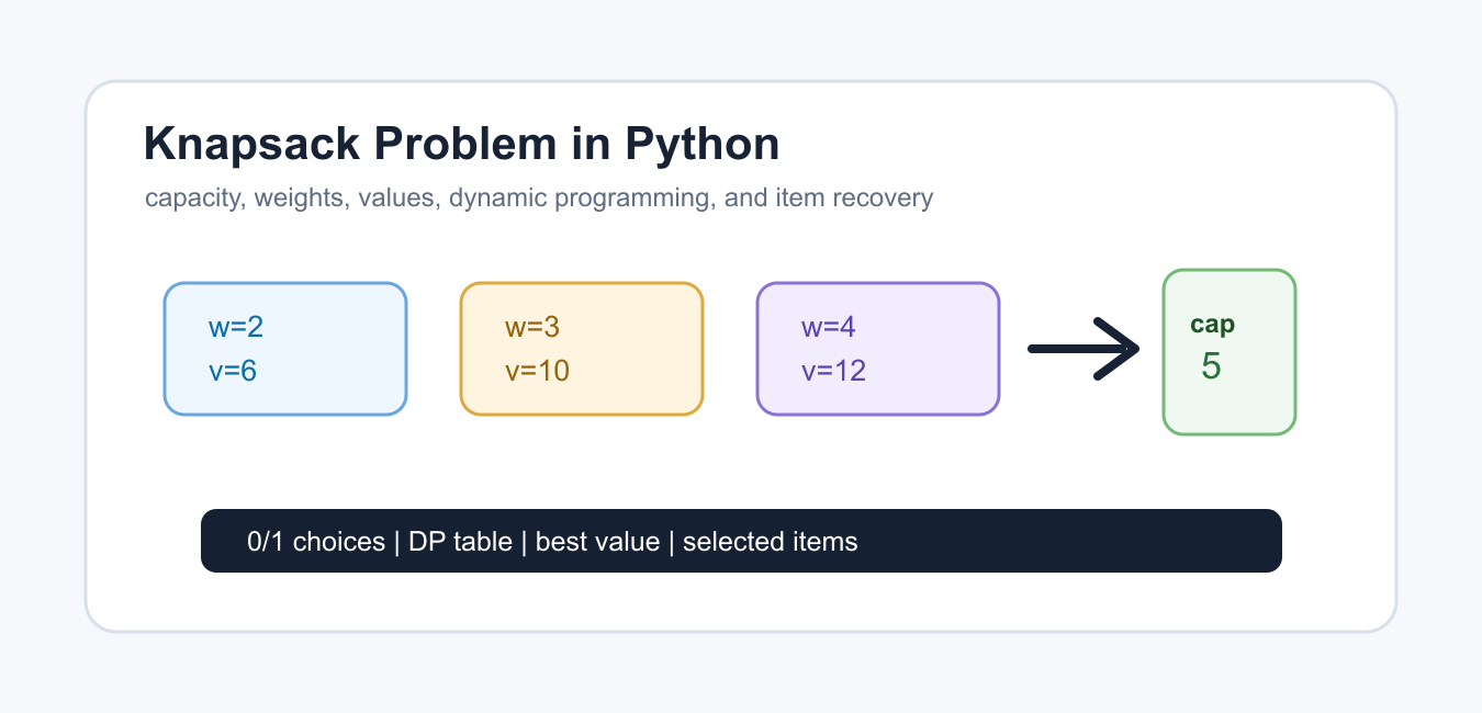
Quick answer: For 0/1 knapsack, dynamic programming evaluates each item against capacities by choosing the better of skipping it or taking it when it fits. The table can reconstruct the selected subset, while greedy value-to-weight selection is not generally optimal.

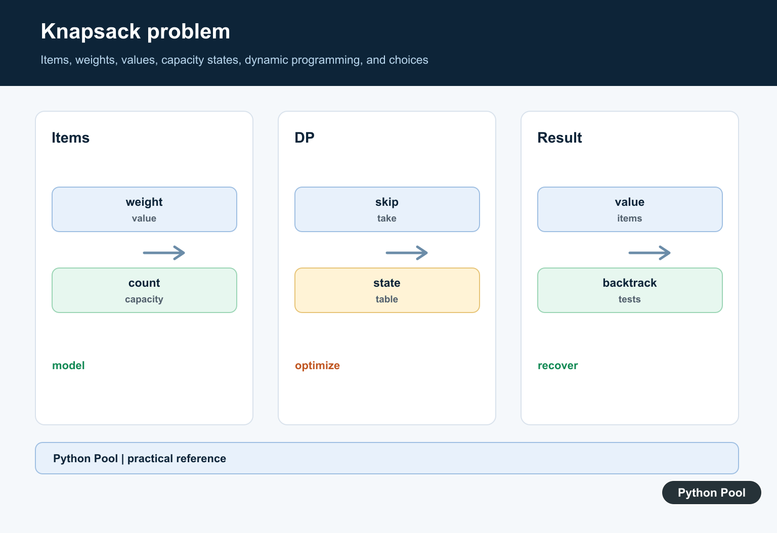
The knapsack problem asks which items to choose when each item has a weight and value, and the bag has a maximum capacity. The common 0/1 version lets you either take an item once or leave it. You cannot split an item.

The official Python documentation covers itertools.combinations() and functools.cache().

For small inputs, brute force is easy to understand. For larger 0/1 inputs with integer weights, dynamic programming is the standard approach. Greedy sorting by value or value per weight can be useful for intuition, but it does not always produce the best 0/1 answer.

Use simple data structures while learning the algorithm. A list of weights, a list of values, and a capacity are enough to demonstrate the core choices.

Make sure the weight and value lists line up by index. If weights[2] is the weight of an item, values[2] should be the value of that same item. In production code, a list of objects or dictionaries can make that relationship clearer.

All examples below use non-negative integer weights. If your weights are decimals, convert to a consistent unit such as grams or cents before using table-based dynamic programming.

Brute Force With Combinations

Brute force tries every possible subset and keeps the best valid value.

from itertools import combinations

weights = [2, 3, 4]
values = [6, 10, 12]
capacity = 5

best_value = 0
best_items = ()

for size in range(len(weights) + 1):
    for items in combinations(range(len(weights)), size):
        total_weight = sum(weights[index] for index in items)
        total_value = sum(values[index] for index in items)
        if total_weight <= capacity and total_value > best_value:
            best_value = total_value
            best_items = items

print(best_value)
print(best_items)

This finds the optimal result, but it checks many subsets. The number of subsets doubles with each added item.

Use brute force for tiny examples, tests, and validation of another implementation. It is too slow for large item lists.

Its main advantage is confidence. Because it tries every subset, it is a helpful way to verify that a dynamic programming implementation returns the same answer on small cases.

Dynamic Programming Table

A bottom-up dynamic programming table stores the best value for each prefix of items and each capacity.

weights = [2, 3, 4]
values = [6, 10, 12]
capacity = 5
n = len(weights)

dp = [[0] * (capacity + 1) for _ in range(n + 1)]

for item in range(1, n + 1):
    weight = weights[item - 1]
    value = values[item - 1]
    for limit in range(capacity + 1):
        dp[item][limit] = dp[item - 1][limit]
        if weight <= limit:
            dp[item][limit] = max(
                dp[item][limit],
                value + dp[item - 1][limit - weight],
            )

print(dp[n][capacity])

This returns the best value without listing every subset. The table has items + 1 rows and capacity + 1 columns.

This method works well when weights and capacity are non-negative integers and the capacity is not enormous.

The time and memory cost depend on number_of_items * capacity. A capacity of 50 is easy; a capacity in the millions may need a different strategy or a scaled representation.

Recover Selected Items

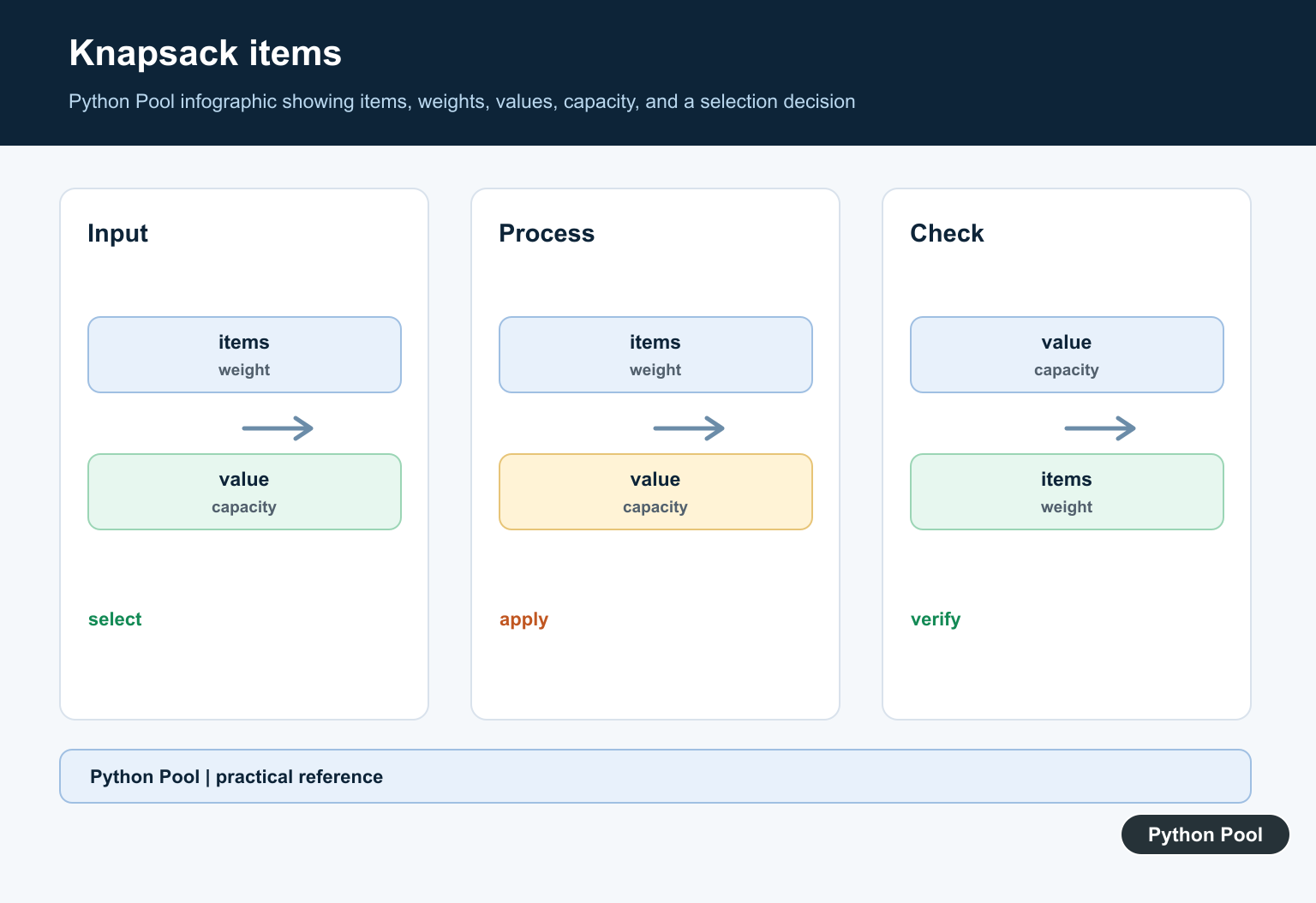
The table can also show which items were chosen. Walk backward through the table and compare each row with the row above it.

weights = [2, 3, 4]
values = [6, 10, 12]
capacity = 5
n = len(weights)
dp = [[0] * (capacity + 1) for _ in range(n + 1)]

for item in range(1, n + 1):
    for limit in range(capacity + 1):
        dp[item][limit] = dp[item - 1][limit]
        if weights[item - 1] <= limit:
            dp[item][limit] = max(
                dp[item][limit],
                values[item - 1] + dp[item - 1][limit - weights[item - 1]],
            )

chosen = []
limit = capacity
for item in range(n, 0, -1):
    if dp[item][limit] != dp[item - 1][limit]:
        chosen.append(item - 1)
        limit -= weights[item - 1]

print(dp[n][capacity])
print(list(reversed(chosen)))

If the value changed from the previous row, the item was used. Subtract its weight and continue upward.

This is useful when the caller needs the actual item indexes, not just the best value.

In a real program, you can map those indexes back to item names, IDs, or records. Keeping indexes in the algorithm keeps the DP table compact.

Use Memoized Recursion

Top-down recursion with caching expresses the choice directly: skip the current item or take it if it fits.

from functools import cache

weights = [2, 3, 4]
values = [6, 10, 12]
capacity = 5

@cache
def best(index, remaining):
    if index == len(weights):
        return 0
    skip = best(index + 1, remaining)
    take = 0
    if weights[index] <= remaining:
        take = values[index] + best(index + 1, remaining - weights[index])
    return max(skip, take)

print(best(0, capacity))

The cache prevents the same subproblem from being solved repeatedly. This version is compact and maps closely to the decision tree.

For very large inputs, an iterative table can be easier to inspect and can avoid recursion-depth concerns.

The memoized form is still excellent for teaching because the two choices are visible: skip the item, or take it and reduce the remaining capacity.

Space-Optimized DP

When you only need the best value, a one-dimensional table can reduce memory use.

weights = [2, 3, 4]
values = [6, 10, 12]
capacity = 5

dp = [0] * (capacity + 1)

for weight, value in zip(weights, values):
    for limit in range(capacity, weight - 1, -1):
        dp[limit] = max(dp[limit], value + dp[limit - weight])

print(dp[capacity])

The inner loop goes backward so each item is used at most once. Forward iteration would turn this into an unbounded-style update.

This is a good production choice when memory matters and selected-item recovery is not required.

If selected items are needed with a one-dimensional table, store extra backtracking information or rerun a separate recovery step. That extra complexity is why the full table is often better for explanations.

Greedy Can Be Wrong

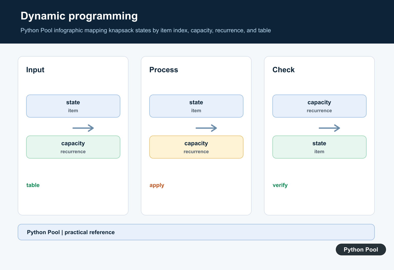
Sorting by value-to-weight ratio is tempting, but it can fail for the 0/1 knapsack problem.

weights = [10, 20, 30]
values = [60, 100, 120]
capacity = 50

greedy_items = [0, 1]
optimal_items = [1, 2]

print(sum(values[i] for i in greedy_items))
print(sum(values[i] for i in optimal_items))

The greedy choice gives value 160, but the better 0/1 answer gives 220. Greedy methods are not a substitute for DP when the exact optimum is required.

Greedy methods do solve related fractional versions where items can be split. That is a different problem from 0/1 knapsack, where every item is either taken whole or skipped.

The practical rule is simple: brute force is best for tiny verification cases, dynamic programming is the standard exact solution for integer capacities, memoized recursion is readable, and one-dimensional DP is memory efficient.

Good tests should include empty item lists, zero capacity, one item that fits, one item that does not fit, ties, and cases where greedy selection fails.

Define The Variant

Clarify whether each item can be used once, repeatedly, or fractionally. The recurrence and algorithm change across 0/1, unbounded, and fractional knapsack, so do not mix their solutions.

Build Capacity States

Let dp[i] represent the best value using the first i items and capacity c. For an item that fits, compare the state that skips it with the state that takes its value and remaining capacity.

Reduce Memory When Needed

If only the best value is required, a one-dimensional table can update capacities in descending order for 0/1 knapsack. Descending order prevents the same item from being used twice in one pass.

Reconstruct The Choices

Keep a decision table or walk backward comparing adjacent states. When a state changes because an item was taken, subtract its weight and continue with the prior item.

Check Complexity And Capacity

The common O(nC) approach is pseudo-polynomial because it depends on numeric capacity. For huge capacities, consider value-based dynamic programming, meet-in-the-middle, approximation, or a domain-specific solver.

Test Against Brute Force

Test empty items, zero capacity, overweight items, ties, duplicate weights, negative or invalid values, and a small brute-force reference. Assert both optimum value and selected indices when reconstruction is required.

Use the official itertools documentation for small brute-force comparisons. Related Python Pool references include lists and tests.

For related algorithm design, compare state and item lists, brute-force tests, and decision metadata when solving knapsack.

Frequently Asked Questions

What is the 0/1 knapsack problem?

Choose each item at most once to maximize total value without exceeding a capacity limit.

Why does a greedy value-to-weight rule fail?

Local ratios can block a better combination, so greedy selection is not generally optimal for 0/1 knapsack.

What is the dynamic-programming complexity?

The common table solution is O(nC) time and O(nC) space, or O(C) space when only the best value is needed.

How do I reconstruct the chosen items?

Store decisions or compare adjacent states while walking backward through the table to identify which items were taken.