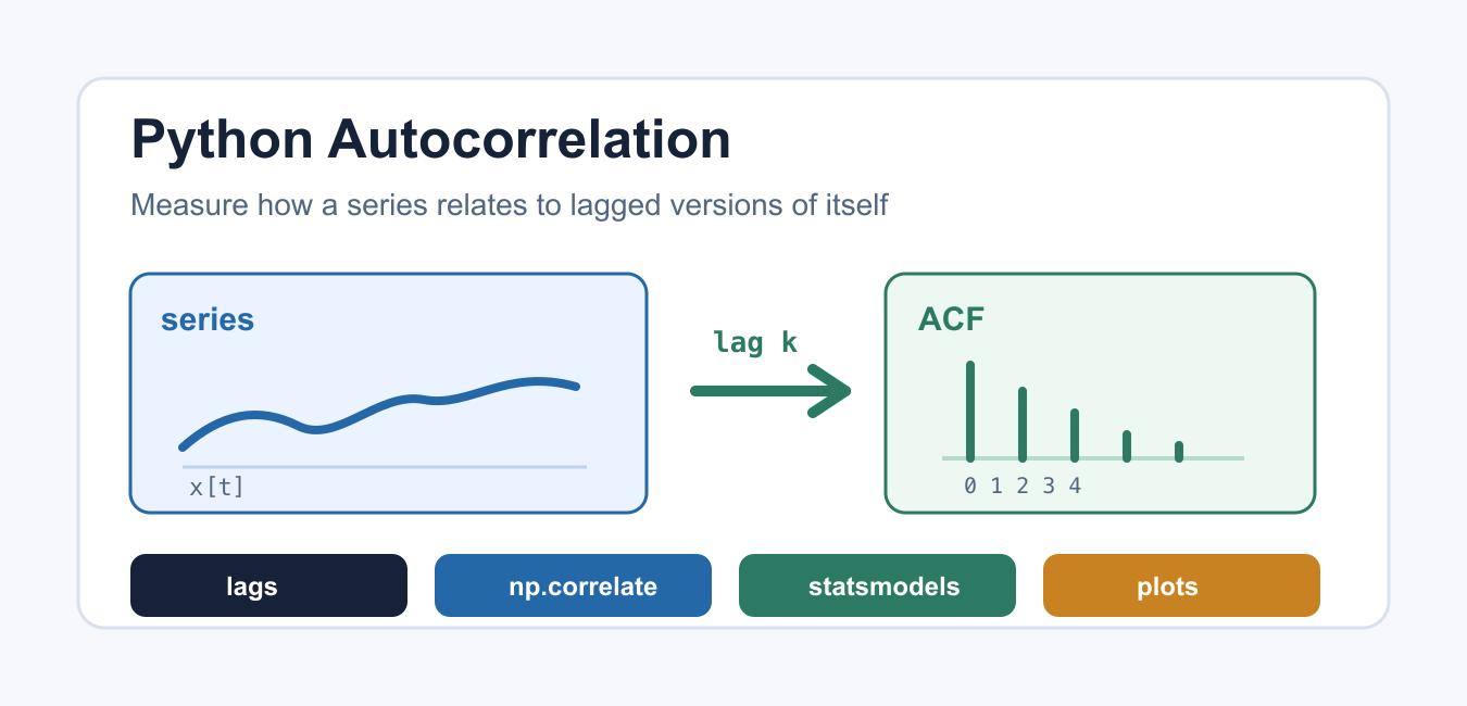
Quick answer: Autocorrelation compares a centered time series with a lagged copy under a chosen normalization. State the lag sign, denominator, missing-value handling, detrending, and confidence method before comparing results across Python libraries.
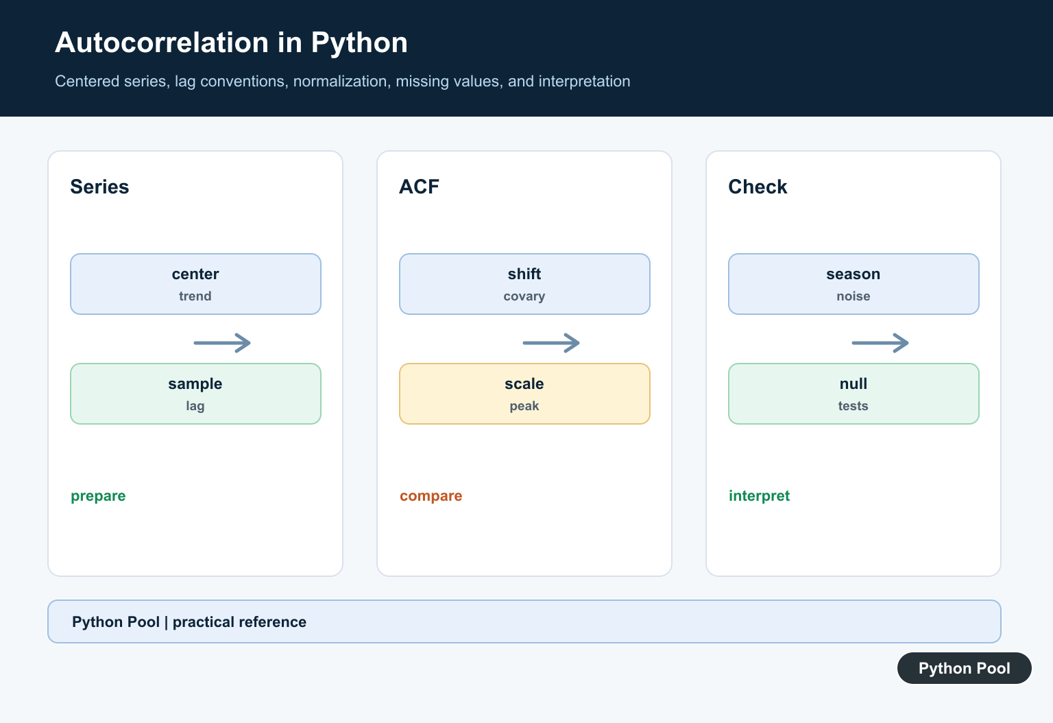
Python autocorrelation measures how a series relates to lagged versions of itself. In time-series analysis, it helps answer questions such as whether today’s value is related to yesterday’s value, whether a signal has repeating structure, or whether model residuals still contain pattern.
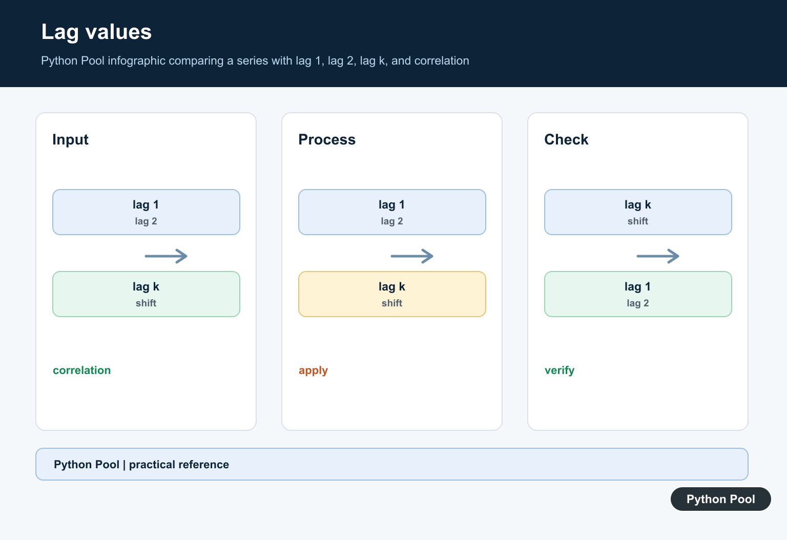
Autocorrelation is usually reported by lag. Lag 1 compares each value with the previous value. Lag 2 compares values two steps apart, and so on. A high positive autocorrelation means nearby values tend to move together; a negative value means they tend to move in opposite directions.
Before calculating autocorrelation, make sure the data order is meaningful. It is useful for time series, signals, sensor readings, and ordered observations. It is not useful for a shuffled list where neighboring values have no natural relationship.
Autocorrelation With NumPy
NumPy provides np.correlate(), which can compute correlation-like sums for one-dimensional sequences. For autocorrelation, subtract the mean first so the comparison is centered around zero.
import numpy as np

x = np.array([3, 4, 6, 8, 7, 5], dtype=float)
centered = x - x.mean()
raw = np.correlate(centered, centered, mode="full")

autocovariance = raw[raw.size // 2:]
print(autocovariance)
The second half of the full result contains lag 0, lag 1, lag 2, and later lags. Lag 0 is the series compared with itself, so it is the largest value in many examples. The centered data step is important because otherwise the level of the series can dominate the result.
Normalize the Result
Raw autocovariance values are harder to compare across datasets. Divide by the lag-0 value to get autocorrelation values where lag 0 is 1.
import numpy as np

x = np.array([3, 4, 6, 8, 7, 5], dtype=float)
centered = x - x.mean()
raw = np.correlate(centered, centered, mode="full")
autocovariance = raw[raw.size // 2:]

autocorrelation = autocovariance / autocovariance[0]
print(np.round(autocorrelation, 3))
For related array basics, see NumPy arrays, Python averages, and NumPy round. Normalization is especially helpful when comparing multiple series that have different units or different variance.
Use statsmodels acf()
For time-series work, statsmodels.tsa.stattools.acf() is often more convenient. It returns autocorrelation values directly and supports options for missing data, confidence intervals, and FFT-based calculation.
import numpy as np
from statsmodels.tsa.stattools import acf

x = np.array([3, 4, 6, 8, 7, 5], dtype=float)
values = acf(x, nlags=3, fft=False)

print(np.round(values, 3))
Use statsmodels when you are already doing forecasting, residual diagnostics, or statistical time-series analysis. Use the simple NumPy version when you want to understand the calculation or avoid another dependency. In production analysis, statsmodels is also useful because it makes common statistical choices explicit.
Plot an Autocorrelation Function
An ACF plot shows autocorrelation by lag. A simple stem plot is enough for many notebooks and reports. Matplotlib documents pyplot.stem() for this kind of vertical-line plot.
import numpy as np
import matplotlib.pyplot as plt
from statsmodels.tsa.stattools import acf

x = np.array([3, 4, 6, 8, 7, 5, 4, 6, 9], dtype=float)
values = acf(x, nlags=5, fft=False)
lags = np.arange(len(values))

plt.stem(lags, values)
plt.xlabel("Lag")
plt.ylabel("Autocorrelation")
plt.grid(True, alpha=0.3)
plt.show()
For plot styling and exports, see Python Pool’s guides to Matplotlib grid lines and saving Matplotlib figures. Label the lag axis clearly so readers know whether lag means hours, days, rows, or another interval.
How to Interpret Autocorrelation
Autocorrelation near 1 means the series has strong positive similarity at that lag. Values near 0 mean little linear relationship at that lag. Negative values mean the series tends to move in opposite directions at that lag.
acf_values = np.array([1.0, 0.72, 0.34, -0.05, -0.22])

for lag, value in enumerate(acf_values):
    print(f"lag {lag}: {value:.2f}")
Interpretation depends on the domain. A lag-7 pattern may matter for daily traffic because it can indicate weekly seasonality. A slow decay can suggest trend or persistence. Always combine ACF with domain knowledge and visual inspection of the original series.
Choose a Reasonable Number of Lags
Too many lags can make the plot noisy and misleading. As lag increases, fewer overlapping observations are available, so the estimate becomes less stable. A simple starting point is to inspect only a fraction of the series length.
def max_reasonable_lag(length):
    return max(1, length // 4)

print(max_reasonable_lag(20))
print(max_reasonable_lag(100))
This rule is not universal, but it prevents a small dataset from being stretched into a long, noisy ACF plot. For serious forecasting work, choose lags based on the sampling interval and the seasonality you expect.
Common Mistakes
Do not treat autocorrelation as proof of causation. It only measures how a series relates to lagged versions of itself. Also avoid using too many lags for a small dataset; long-lag estimates can become noisy because fewer overlapping points are available.
If the series has a strong trend, consider differencing, detrending, or using rolling summaries before reading too much into ACF values. For smoothing examples, see moving average in Python. Missing values also need a deliberate policy before calculating autocorrelation.
Conclusion
Python autocorrelation can be calculated directly with np.correlate() or with statsmodels.acf() for time-series workflows. Center the data, normalize the result when comparing lags, and interpret ACF values alongside plots and domain context. Autocorrelation is most useful for detecting persistence, seasonality, and remaining pattern in time-series data.
Center The Series
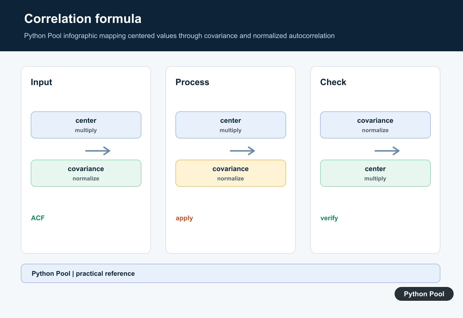
Subtract a mean or another baseline before calculating covariance-like autocorrelation. A trend can produce high correlations that reflect non-stationarity rather than a repeating process.
Define The Lag Convention
At lag k, specify which observations are paired and whether positive k means the series is shifted forward or backward. This affects plots and comparisons even when the magnitude looks similar.
Choose Normalization
Common choices divide by the zero-lag variance, use biased or unbiased denominators, or compute a correlation coefficient on overlapping pairs. Document the choice and its edge cases.
Handle Missing Values
Drop or align missing observations according to a stated rule. Pairwise deletion changes sample size by lag, while imputation can add structure that was not present in the original series.
Interpret With Context
Seasonality, trend, sampling interval, outliers, and changing variance affect the autocorrelation function. Compare against a baseline or null model and avoid reading causality into a correlation curve.
Validate Against A Small Series
Use a hand-computed sequence, white-noise-like simulation, a repeated periodic signal, and constant or short inputs. Compare library outputs with tolerances after matching conventions.
Use the official pandas autocorrelation documentation and statsmodels ACF documentation for library conventions. Related Python Pool references include NumPy arrays and tests.
For related numerical analysis, compare NumPy arrays, lag tests, and series sequences before interpreting autocorrelation.
Frequently Asked Questions
What is autocorrelation?
Autocorrelation measures the relationship between a time series and a lagged version of itself, often after centering and under a chosen normalization convention.
What does a high autocorrelation mean?
It means observations separated by that lag tend to move together under the measure used; interpretation still depends on trend, seasonality, non-stationarity, and sampling.
How do I compute autocorrelation in Python?
Center the series, align it with a shifted copy, compute the lagged covariance or correlation, and document the denominator and missing-value policy.
Why can autocorrelation results differ between libraries?
Libraries may use different lag signs, normalization denominators, missing-value handling, bias corrections, or detrending defaults, so compare conventions as well as numbers.
