Gaussian Elimination in Python: Solve Linear Systems Clearly

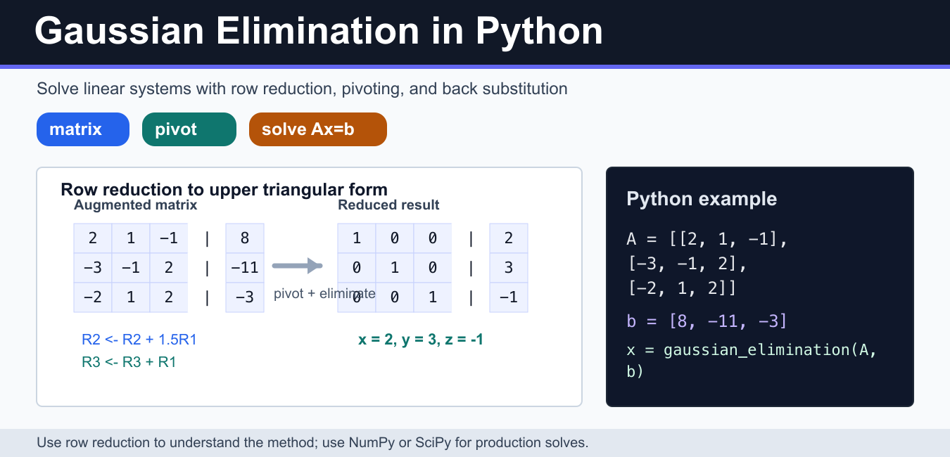
Quick answer: Gaussian elimination applies row operations to an augmented matrix until the system is triangular or reduced, then solves by back substitution. Pivoting, tolerances, singularity checks, and dtype choices determine whether an implementation is reliable.

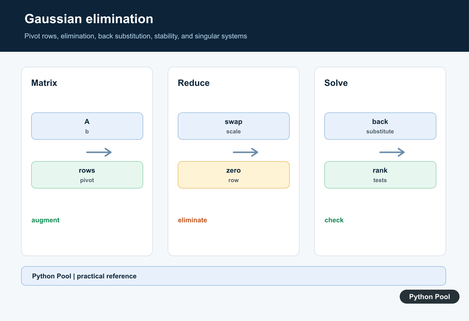
Gaussian elimination is a row-reduction method for solving a linear system such as Ax = b. It transforms an augmented matrix into an easier form by swapping rows, scaling rows, and adding multiples of one row to another. After the matrix is upper triangular, back substitution gives the unknown values.

Use a hand-written implementation when you are learning the method. For production numerical work, prefer numpy.linalg.solve() or scipy.linalg.solve(). Those libraries use battle-tested linear algebra routines and handle many numerical details better than a tutorial implementation.

Gaussian elimination example

Consider this system of equations:

• 2x + y - z = 8
• -3x - y + 2z = -11
• -2x + y + 2z = -3

The coefficient matrix is A, and the right-hand side is b. Gaussian elimination works on the augmented matrix [A | b]. The first phase eliminates values below each pivot. The second phase solves the variables from bottom to top.

Pure Python Gaussian elimination with pivoting

The implementation below uses partial pivoting. For each column, it chooses the row with the largest absolute pivot value and swaps that row into position. Pivoting reduces avoidable division problems and catches singular or nearly singular systems earlier.

def gaussian_elimination(a, b):
    n = len(a)
    matrix = [list(map(float, row)) + [float(rhs)] for row, rhs in zip(a, b)]

    for col in range(n):
        pivot_row = max(range(col, n), key=lambda row: abs(matrix[row][col]))
        if abs(matrix[pivot_row][col]) < 1e-12:
            raise ValueError("the matrix is singular or nearly singular")

        matrix[col], matrix[pivot_row] = matrix[pivot_row], matrix[col]
        pivot = matrix[col][col]

        for j in range(col, n + 1):
            matrix[col][j] /= pivot

        for row in range(col + 1, n):
            factor = matrix[row][col]
            for j in range(col, n + 1):
                matrix[row][j] -= factor * matrix[col][j]

    solution = [0.0] * n
    for row in range(n - 1, -1, -1):
        solution[row] = matrix[row][n] - sum(
            matrix[row][col] * solution[col] for col in range(row + 1, n)
        )

    return solution

This function is intentionally explicit. It builds an augmented matrix, performs elimination, normalizes each pivot row, and then runs back substitution. If you want to display the rows during teaching or debugging, the Matplotlib table guide can help present intermediate matrices.

Run the solver

Now pass the coefficient matrix and right-hand side vector into the function. For this example, the solution is x = 2, y = 3, and z = -1.

a = [
    [2, 1, -1],
    [-3, -1, 2],
    [-2, 1, 2],
]
b = [8, -11, -3]

solution = gaussian_elimination(a, b)
print(solution)

Solve the same system with NumPy

For real numeric work, do not reimplement Gaussian elimination unless you have a specific reason. NumPy solves the same system directly with np.linalg.solve(). It expects a square coefficient matrix and a compatible right-hand side.

import numpy as np

a = np.array(
    [
        [2, 1, -1],
        [-3, -1, 2],
        [-2, 1, 2],
    ],
    dtype=float,
)
b = np.array([8, -11, -3], dtype=float)

solution = np.linalg.solve(a, b)
print(solution)

After solving, a useful check is the residual A @ x - b. A small residual means the computed solution fits the original equations closely. Python’s floating-point arithmetic behavior explains why small rounding differences are normal.

residual = a @ solution - b
print(residual)
print(np.linalg.norm(residual))

Detect singular systems

A singular matrix does not have a unique solution. A row of zeros during elimination, or a pivot close to zero, is a warning sign. NumPy raises LinAlgError for singular systems. PythonPool has a dedicated guide for LinAlgError: Singular Matrix in Python and NumPy.

In teaching code, raising ValueError when the pivot is close to zero is usually enough. In production, use NumPy or SciPy and decide how your application should handle no solution, infinitely many solutions, or ill-conditioned matrices.

Reduced row echelon form with SymPy

If you want symbolic row reduction rather than floating-point numeric solving, SymPy can compute reduced row echelon form with Matrix.rref(). This is useful in algebra lessons because it exposes the row-reduction result directly.

from sympy import Matrix

augmented = Matrix(
    [
        [2, 1, -1, 8],
        [-3, -1, 2, -11],
        [-2, 1, 2, -3],
    ]
)

reduced, pivot_columns = augmented.rref()
print(reduced)
print(pivot_columns)

When to use Gaussian elimination

• Learning linear algebra: implement the algorithm to understand row operations and pivots.
• Small systems: pure Python is fine for demonstrations and tests.
• Large numeric systems: use NumPy or SciPy instead of tutorial code.
• Symbolic math: use SymPy when exact fractions and row echelon form matter.
• Data science workflows: linear algebra appears in optimization, regression, and many algorithms; see PythonPool’s top algorithms for data science overview for broader context.

Numerical notes for Gaussian elimination

Gaussian elimination is straightforward on paper, but computer arithmetic introduces rounding. Partial pivoting helps because it avoids dividing by a tiny pivot when a better row is available. It does not make every system safe, though. Ill-conditioned matrices can still magnify small input errors into large output changes. That is another reason to use NumPy or SciPy for serious calculations.

When checking a solution, multiply the coefficient matrix by the result vector and compare it with the original right-hand side. In NumPy code, the @ operator performs matrix multiplication; PythonPool has a separate guide to the Python @ symbol if you want the syntax background.

References

• NumPy linalg.solve
• SciPy linalg.solve
• SymPy Matrix.rref
• Python floating-point arithmetic
• Gaussian elimination overview

Build The Augmented Matrix

Represent A and b with compatible dimensions and keep the original inputs available for validation. A shape check should reject a non-square or mismatched system before row operations begin.

Choose A Pivot

At each column, select a suitable row and swap it into the pivot position. Partial pivoting is a practical baseline for reducing numerical error when a pivot is small.

Eliminate Below The Pivot

Scale the pivot row or compute factors, then remove the current column from later rows. Avoid exact zero comparisons for floating-point values; use a scale-aware tolerance.

Back-Substitute

Once the matrix is upper triangular, solve from the last row upward and subtract already-known terms. Check the residual A @ x – b rather than trusting a plausible-looking vector.

Handle Singular And Ill-Conditioned Systems

A zero or tiny pivot can indicate no unique solution, an underdetermined system, or numerical instability. Use rank and condition diagnostics, or delegate to a tested library routine.

Compare With NumPy

For production work, numpy.linalg.solve or a specialized factorization is usually safer and faster than an educational implementation. Keep a small manual version as a reference test where useful.

The official NumPy solve documentation covers solving full-rank systems. Related Python Pool references include NumPy arrays and tests.

For related linear algebra, compare NumPy matrix arrays, residual tests, and row operations before solving a system.

Frequently Asked Questions

What is Gaussian elimination?

It is a sequence of row operations that transforms a linear system into a form that can be solved by back substitution or further reduction.

Why is pivoting important?

Swapping rows to use a better pivot can reduce numerical error and avoid dividing by a zero or very small value.

When should I use NumPy instead of a manual implementation?

Use a tested linear-algebra routine for production numerical work; implement the algorithm manually for learning, controlled transformations, or specialized needs.

How do I detect a singular system?

Monitor pivot magnitudes and matrix rank or solver errors, while using a tolerance appropriate to the scale and dtype of the input.