
Quick answer: A* uses g, the cost already traveled, plus h, a heuristic estimate to the goal, to prioritize nodes. With an admissible heuristic and consistent graph assumptions, it can find an optimal path while exploring less toward the target than uninformed Dijkstra search.
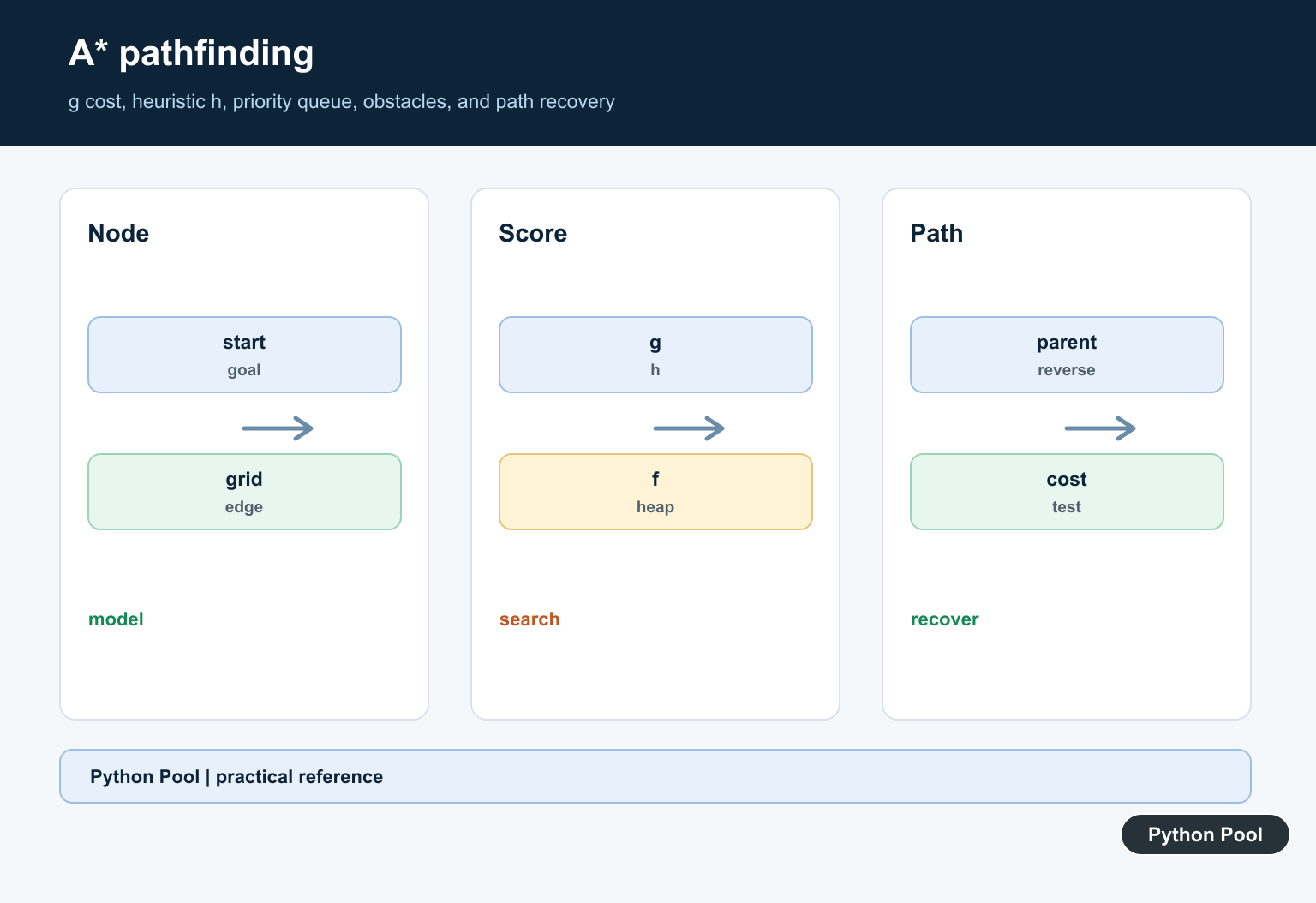
The A* algorithm finds a low-cost path from a start node to a goal node by combining the cost already paid with a heuristic estimate of the cost still remaining. In pathfinding, the usual score is f(n) = g(n) + h(n). The g score is the known cost from the start to the current node, and the h score is the estimated cost from the current node to the goal. A* uses a heuristic to expand one promising path, while Python Genetic Algorithm Guide searches with a population, fitness scores, crossover, and mutation.
A* is useful for grid maps, navigation, puzzle solving, game AI, and weighted graph search. It behaves like Dijkstra’s algorithm when the heuristic is zero, and it becomes more directed when the heuristic gives useful guidance. For comparison with a no-heuristic shortest-path algorithm, see the Dijkstra’s algorithm in Python guide.
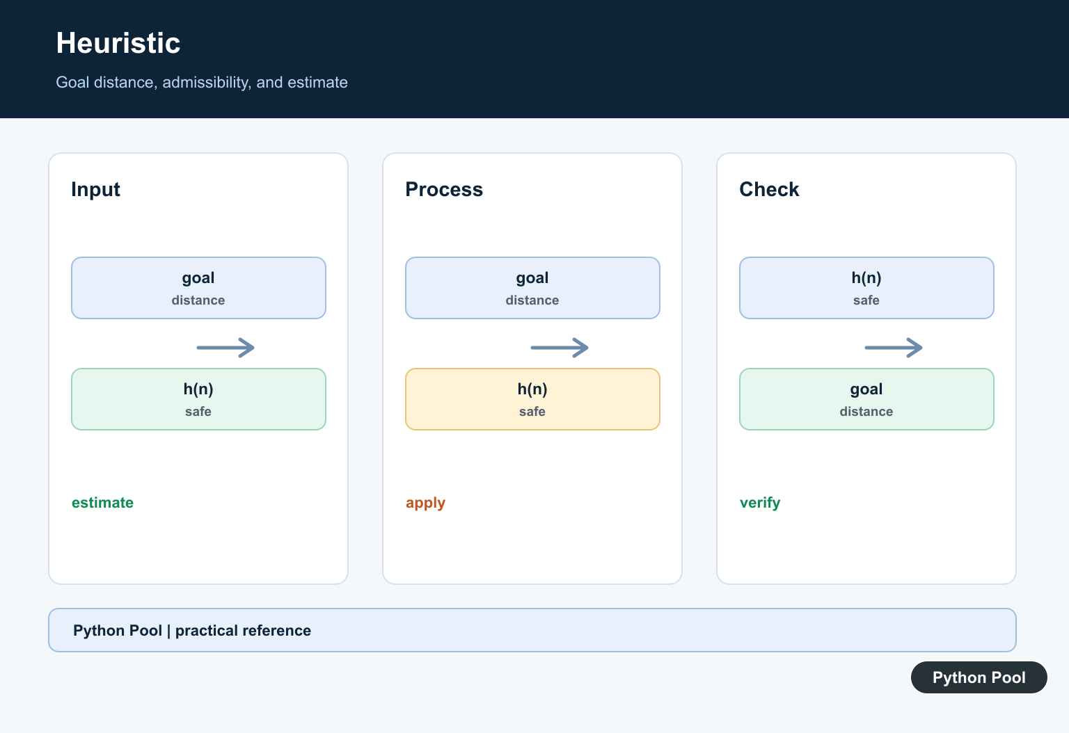
The quality of A* depends on the heuristic. A heuristic is admissible when it never overestimates the remaining cost. On a four-direction grid with equal movement cost, Manhattan distance is a common choice. The Python heapq documentation is also relevant because a priority queue is the normal way to process the lowest-score node first.
Most implementations keep two ideas in mind: the open set contains nodes that may still lead to a better path, and the recorded scores prevent the algorithm from accepting a worse route to the same node. A priority queue makes this efficient because the next node to expand is always the one with the lowest estimated total cost.
Define The Heuristic
For a grid where movement is allowed up, down, left, and right, Manhattan distance counts how many row and column steps separate two cells.
from heapq import heappop, heappush


def manhattan(a, b):
    row_a, col_a = a
    row_b, col_b = b
    return abs(row_a - row_b) + abs(col_a - col_b)
This function returns an estimate, not the final path cost. It is fast to calculate and works well when diagonal movement is not allowed.
If diagonal movement is allowed, use a heuristic that matches that movement model. A mismatch can still find a path, but it may explore more nodes or lose the shortest-path guarantee if the estimate is too optimistic or too large.
Find Walkable Neighbor Cells
The neighbor function controls which cells can be explored. In this example, 0 means open space and 1 means a blocked cell.
def walkable_neighbors(grid, node):
    row, col = node
    moves = [(1, 0), (-1, 0), (0, 1), (0, -1)]

    for row_step, col_step in moves:
        next_row = row + row_step
        next_col = col + col_step
        inside_rows = 0 <= next_row < len(grid)
        inside_cols = 0 <= next_col < len(grid[0])
        if inside_rows and inside_cols and grid[next_row][next_col] == 0:
            yield (next_row, next_col)
Changing this function changes the search space. For diagonal movement, add diagonal offsets and adjust the movement cost so the heuristic remains consistent.
Rebuild The Final Path
A* stores the best previous node for each visited node. Once the goal is reached, walk backward through that mapping and reverse the result.
def rebuild_path(came_from, current):
    path = [current]
    while current in came_from:
        current = came_from[current]
        path.append(current)
    path.reverse()
    return path
This keeps path construction separate from search. The search loop can focus on scores, while the rebuild helper handles the final route.
Implement A* With heapq
The priority queue stores nodes by estimated total cost. Each time the loop runs, it expands the node with the smallest f score.
def a_star(grid, start, goal):
    open_heap = []
    heappush(open_heap, (0, start))
    came_from = {}
    g_score = {start: 0}

    while open_heap:
        _, current = heappop(open_heap)
        if current == goal:
            return rebuild_path(came_from, current)

        for neighbor in walkable_neighbors(grid, current):
            tentative_g = g_score[current] + 1
            if tentative_g < g_score.get(neighbor, float("inf")):
                came_from[neighbor] = current
                g_score[neighbor] = tentative_g
                f_score = tentative_g + manhattan(neighbor, goal)
                heappush(open_heap, (f_score, neighbor))

    return []
The dictionary named g_score records the best known cost to each node. If the algorithm finds a cheaper route to a node, it updates the route and pushes the node back into the priority queue.
This version may push the same node more than once when a better path is found later. That is acceptable for a compact implementation because the best score is still stored in g_score. Larger systems often add more bookkeeping to skip stale queue entries.
Run A* On A Grid
This grid has a wall in the middle, so the path must move around blocked cells. The returned list contains grid coordinates from start to goal.
grid = [
    [0, 0, 0, 0],
    [1, 1, 0, 1],
    [0, 0, 0, 0],
    [0, 1, 1, 0],
]

path = a_star(grid, (0, 0), (3, 3))
print(path)
If the function returns an empty list, no path was found under the current movement rules. Check blocked cells, grid bounds, and whether the start or goal cell is blocked.
Small test grids are useful because you can inspect the returned coordinates by eye. Once the path is correct on small maps, the same structure scales to larger maps as long as neighbor generation and movement costs remain consistent.
Use A* On A Weighted Graph
For a weighted graph, neighbors carry edge costs. The heuristic function should estimate the remaining cost for graph nodes rather than grid cells.
def graph_a_star(graph, heuristic, start, goal):
    open_heap = [(0, start)]
    came_from = {}
    g_score = {start: 0}

    while open_heap:
        _, current = heappop(open_heap)
        if current == goal:
            return rebuild_path(came_from, current)

        for neighbor, cost in graph[current]:
            tentative_g = g_score[current] + cost
            if tentative_g < g_score.get(neighbor, float("inf")):
                came_from[neighbor] = current
                g_score[neighbor] = tentative_g
                heappush(open_heap, (tentative_g + heuristic(neighbor), neighbor))

    return []
This version works for route maps, game areas, and abstract graph search as long as edge costs are non-negative. If the heuristic overestimates, A* may lose its shortest-path guarantee. If you do not have a meaningful heuristic, use Dijkstra’s algorithm instead.
For weighted graphs, the heuristic should use the same cost scale as the edges. If edge weights represent time, estimate remaining time. If edge weights represent distance, estimate remaining distance.
The A* algorithm is effective because it balances explored cost and estimated remaining cost. Keep the heuristic simple, use a priority queue for the open set, store previous nodes for path rebuilding, and test the implementation on small maps before using it in larger pathfinding systems. A* scores routes toward an explicit goal, while Viterbi Algorithm in Python Guide keeps the best hidden-state path for each observation step.
Represent The Search State
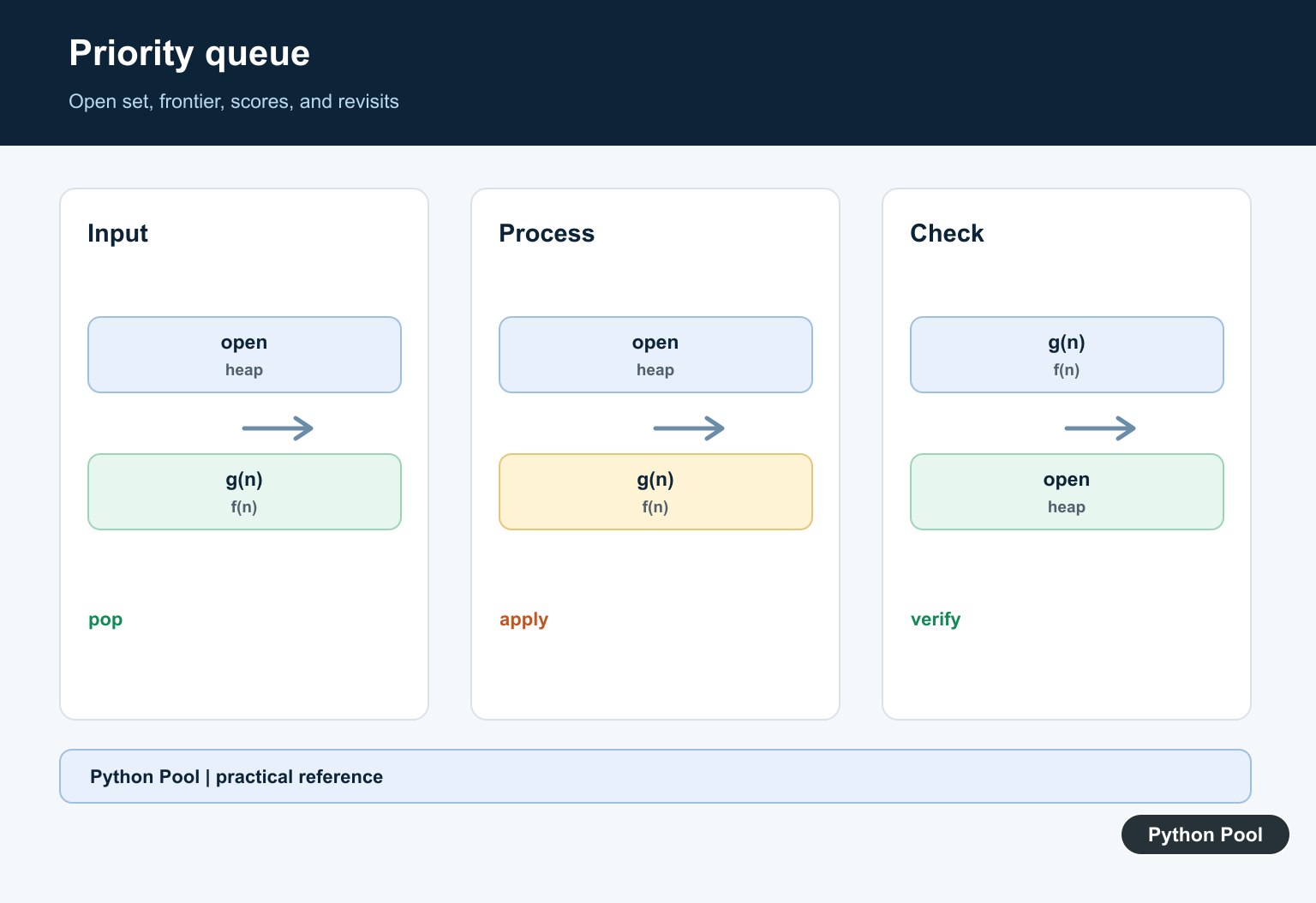
Keep a priority queue, best-known g scores, and predecessor links. A node’s priority is f = g + h, while the predecessor map is used later to reconstruct the path.
Choose The Heuristic
Manhattan distance suits four-direction grids with uniform costs, while Euclidean distance can suit movement with diagonals. The heuristic must not overestimate the remaining cost when optimality is required.
Handle Stale Queue Entries
Like heap-based Dijkstra, A* may push a node more than once when a better path is found. Skip entries that no longer match the current best g score instead of assuming the queue has decrease-key support.
Model Obstacles And Neighbors
Generate only valid, in-bounds neighbors and define the movement cost for each. Do not allow diagonal corner cutting unless the domain explicitly permits it.
Separate Optimality From Speed
A stronger but inadmissible heuristic may find a path faster but can lose optimality. Choose the tradeoff intentionally and document whether the result must be shortest or merely acceptable.
Test Path Contracts
Test start equals goal, blocked goals, unreachable areas, ties, weighted edges, obstacles, and an empty grid. Assert path validity, cost, and optimality against a small reference graph.
The official heapq documentation covers the priority queue primitive. Related Python Pool references include Dijkstra and tests.
For related pathfinding, compare Dijkstra search, graph tests, and priority queues when implementing A*.
Frequently Asked Questions
What is the A* algorithm?
A* is a graph-search algorithm that uses path cost so far and a heuristic estimate to find efficient paths toward a goal.
What makes an A* heuristic admissible?
It never overestimates the true remaining cost, which preserves optimality under the algorithm’s assumptions.
How is A* different from Dijkstra?
Dijkstra uses no goal-directed heuristic, while A* adds h to prioritize nodes that appear closer to the target.
How do I reconstruct an A* path?
Store a predecessor when a node’s best path improves, then follow predecessors from the goal back to the start and reverse the sequence.

great