Matplotlib Circle: patches.Circle, Radius, Aspect Ratio, and Geometry

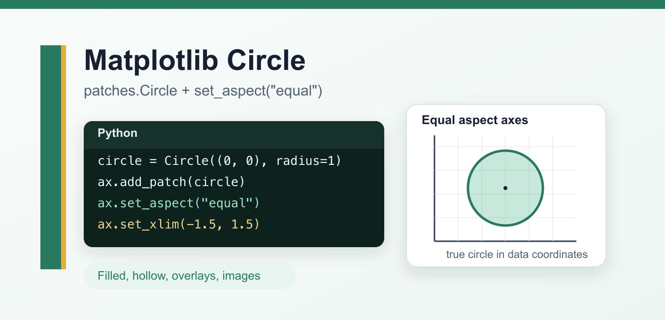
Quick answer: Use matplotlib.patches.Circle when the goal is a true geometric circle on an Axes. Add the patch, set x and y limits so it is visible, and use an equal aspect ratio when one unit on the x-axis must have the same screen size as one unit on the y-axis. A point-by-point parametric curve is useful when you need sampled coordinates instead.

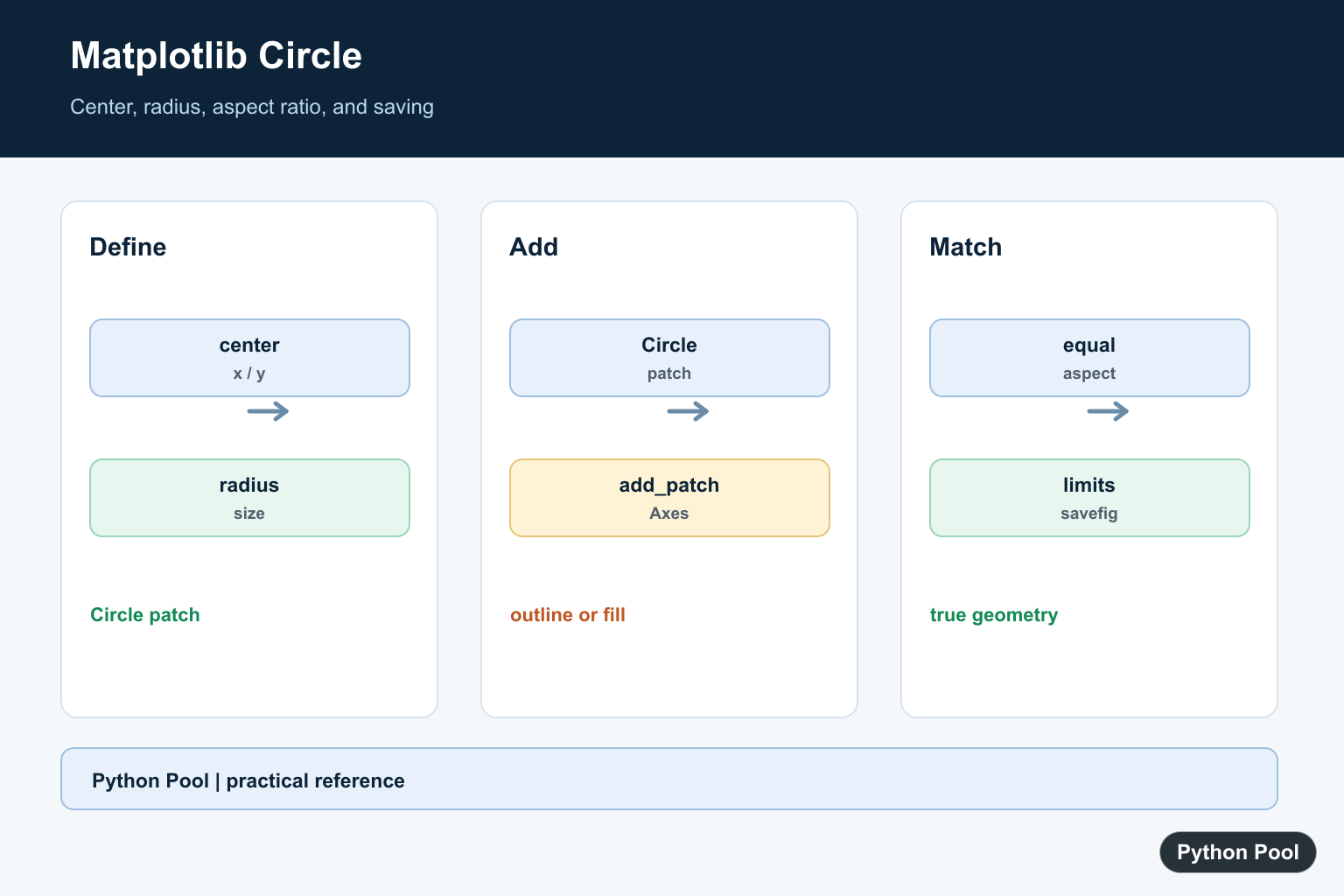
There are two common ways to draw a circle in Matplotlib: add a matplotlib.patches.Circle object to an Axes, or plot points generated from the circle equation. For most annotation and drawing tasks, patches.Circle is the cleaner choice because it creates a true circle patch at a center point with a radius.

The key detail is aspect ratio. A mathematically correct circle can look like an oval if the x-axis and y-axis use different scales. Set the Axes aspect to "equal" when the geometry matters. The geometry behind every radius and circumference calculation uses pi; Python math.pi: Use Pi for Circle Calculations shows the corresponding math.pi operations.

Draw a circle with patches.Circle

import matplotlib.pyplot as plt
from matplotlib.patches import Circle

fig, ax = plt.subplots()

circle = Circle((0, 0), radius=1, facecolor="tab:blue", alpha=0.35)
ax.add_patch(circle)

ax.set_xlim(-1.5, 1.5)
ax.set_ylim(-1.5, 1.5)
ax.set_aspect("equal")
ax.grid(True)
plt.show()

Circle((0, 0), radius=1) creates the patch. ax.add_patch(circle) adds it to the Axes. The axis limits are set manually so the patch is visible, and set_aspect("equal") keeps x and y units the same size. When the data is naturally expressed as angles and radii rather than a circle patch, use the polar axes workflow in Matplotlib Polar Plot: pyplot.polar() and Polar Axes.

Hollow circle

Use fill=False when you want only the outline:

import matplotlib.pyplot as plt
from matplotlib.patches import Circle

fig, ax = plt.subplots()

circle = Circle(
    (2, 3),
    radius=1.25,
    fill=False,
    edgecolor="crimson",
    linewidth=3,
)
ax.add_patch(circle)

ax.set_xlim(0, 4)
ax.set_ylim(1, 5)
ax.set_aspect("equal")
plt.show()

This is useful for highlighting a region without covering the data underneath.

Transparent circle over data

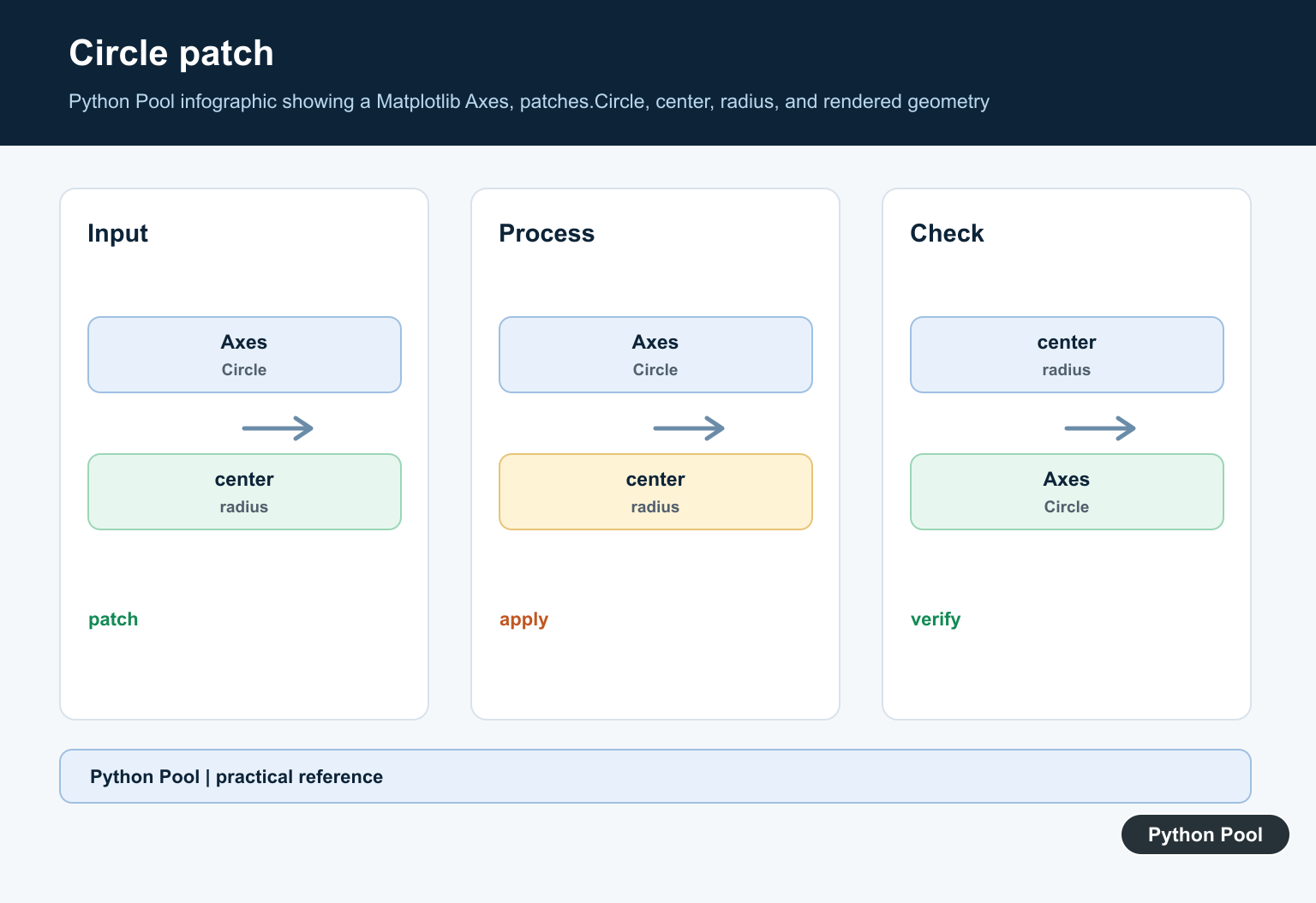
For overlays, set alpha and choose a visible edge color:

import matplotlib.pyplot as plt
from matplotlib.patches import Circle

x = [0, 1, 2, 3, 4]
y = [1, 3, 2, 5, 4]

fig, ax = plt.subplots()
ax.scatter(x, y, color="black")

highlight = Circle((3, 5), radius=0.55, facecolor="gold", edgecolor="orange", alpha=0.35)
ax.add_patch(highlight)

ax.set_aspect("equal", adjustable="datalim")
ax.autoscale_view()
plt.show()

If the circle is added after the data, confirm the limits still include the patch. In many examples it is simpler to set xlim and ylim manually.

Circle from the equation

When you need a circle as a line rather than a patch, generate points from the parametric equation:

import numpy as np
import matplotlib.pyplot as plt

radius = 2
center_x, center_y = 1, -1
theta = np.linspace(0, 2 * np.pi, 300)

x = center_x + radius * np.cos(theta)
y = center_y + radius * np.sin(theta)

fig, ax = plt.subplots()
ax.plot(x, y, color="tab:green")
ax.set_aspect("equal")
ax.grid(True)
plt.show()

This method is useful when you want to style the circle like a plotted curve or combine it with other parametric geometry.

Draw multiple circles

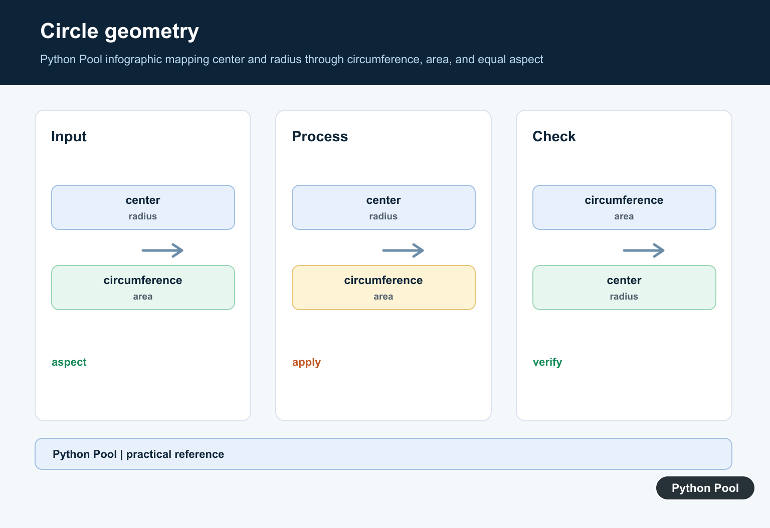
Create one Circle object per circle. Do not reuse the same patch object across different Axes.

import matplotlib.pyplot as plt
from matplotlib.patches import Circle

fig, ax = plt.subplots()

for x, y, r in [(0, 0, 0.4), (1, 0.5, 0.25), (2, 0, 0.6)]:
    ax.add_patch(Circle((x, y), r, fill=False, linewidth=2))

ax.set_xlim(-1, 3)
ax.set_ylim(-1, 1.5)
ax.set_aspect("equal")
plt.show()

For many circles with shared styling, Matplotlib also supports patch collections, but individual patches are easier for small examples.

Draw a circle on an image

You can add a circle patch on top of an image displayed with imshow():

import matplotlib.pyplot as plt
from matplotlib.patches import Circle

img = plt.imread("sample.png")
fig, ax = plt.subplots()
ax.imshow(img)

circle = Circle((120, 80), radius=35, fill=False, edgecolor="red", linewidth=3)
ax.add_patch(circle)

ax.axis("off")
plt.show()

The center and radius are in image pixel coordinates when the image is displayed with the default data coordinates. For more image display examples, see our guide to Matplotlib imshow().

Common mistakes

The circle looks like an oval: Set ax.set_aspect("equal"). Our Matplotlib aspect ratio guide covers this in more detail.

The circle does not appear: Set xlim and ylim so the circle’s center and radius fit inside the visible Axes.

The circle covers data: Use alpha, fill=False, or a lower zorder.

Only circular markers are needed: Use scatter() markers instead of patches. A marker is sized in points, while a Circle patch is sized in data coordinates. For marker options, see our Matplotlib marker guide.

Official references

• Matplotlib documentation for patches.Circle
• Matplotlib documentation for Axes.add_patch()
• Matplotlib documentation for Axes.set_aspect()
• Matplotlib equal-axis aspect ratio example

Conclusion

Use matplotlib.patches.Circle plus ax.add_patch() when you want a circle in data coordinates. Set the axis limits and use ax.set_aspect("equal") so the patch displays as a true circle. Use the parametric equation method when you need a circle as a plotted line, and use scatter markers when you only need circular points.

Keep Circle Geometry Undistorted

A patch stores a center and radius, but the displayed shape also depends on the Axes transform. set_aspect(‘equal’) is the important step for maps, diagrams, measurements, and any plot where a radius should look the same in both directions.

import matplotlib.pyplot as plt
from matplotlib.patches import Circle

fig, ax = plt.subplots()
ax.add_patch(Circle((0, 0), radius=2, facecolor="tab:blue", alpha=0.35))
ax.set_xlim(-3, 3)
ax.set_ylim(-3, 3)
ax.set_aspect("equal")
ax.grid(True)

Draw A Hollow Circle And Label It

Use fill=False when the boundary matters more than the interior. Set edgecolor and linewidth explicitly, then place a text label in data coordinates so the annotation follows the plotted geometry.

import matplotlib.pyplot as plt
from matplotlib.patches import Circle

fig, ax = plt.subplots()
circle = Circle((2, 3), radius=1.25, fill=False, edgecolor="crimson", linewidth=3)
ax.add_patch(circle)
ax.text(2, 3, "center", ha="center", va="center")
ax.set(xlim=(0, 4), ylim=(1, 5), aspect="equal")

Generate Circle Coordinates When Needed

A patch is the clearest drawing primitive, but some calculations need coordinates along the circumference. The parametric equation x = cx + r cos(theta), y = cy + r sin(theta) creates sampled points that can be plotted or passed to another algorithm.

import numpy as np
import matplotlib.pyplot as plt

theta = np.linspace(0, 2 * np.pi, 200)
cx, cy, radius = 1.0, -1.0, 2.0
x = cx + radius * np.cos(theta)
y = cy + radius * np.sin(theta)

fig, ax = plt.subplots()
ax.plot(x, y, color="tab:orange")
ax.set_aspect("equal")

Save A Reproducible Figure

Set limits and aspect before saving. Use a stable output filename, an explicit format or dpi when the image is part of a report, and close the figure in scripts that create many plots so figures do not accumulate in memory.

from pathlib import Path
import matplotlib.pyplot as plt
from matplotlib.patches import Circle

fig, ax = plt.subplots(figsize=(4, 4))
ax.add_patch(Circle((0, 0), 1, color="tab:green", alpha=0.4))
ax.set(xlim=(-1.5, 1.5), ylim=(-1.5, 1.5), aspect="equal")
path = Path("circle.png")
fig.savefig(path, dpi=160, bbox_inches="tight")
plt.close(fig)
print(path)

Matplotlib documents patches.Circle as a true circle patch and Axes.add_patch() as the method for adding it to an Axes. Related references include aspect ratio, polar plots, and math.pi.

For clipped annotations, check the Axes limits and artist clipping settings before assuming the radius calculation is wrong. The data can be correct while the visible portion is outside the current view.

For related geometric plotting, compare aspect ratio, polar coordinates, and math.pi when choosing between a patch, sampled curve, and measurement formula.

Frequently Asked Questions

How do I draw a circle in Matplotlib?

Create matplotlib.patches.Circle with a center and radius, add it to an Axes with ax.add_patch(), and set limits so the patch is visible.

Why does my Matplotlib circle look like an oval?

The axes may use different scales; call ax.set_aspect(‘equal’) or choose an equivalent box aspect when the geometry must remain circular.

How do I draw a hollow circle?

Pass fill=False and set edgecolor and linewidth on patches.Circle, then add the patch to the Axes.

Can I save a Matplotlib circle figure?

Yes. Configure the limits and aspect first, then call fig.savefig() with a suitable filename and format.