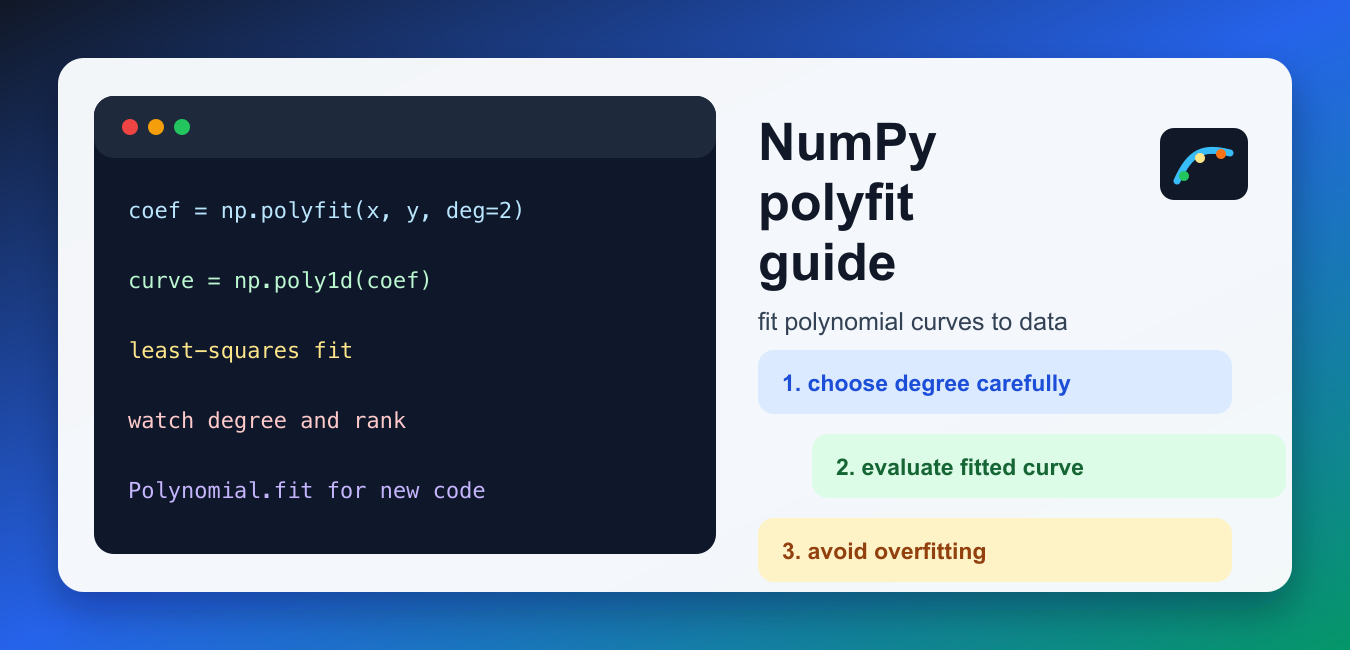
NumPy polyfit() finds polynomial coefficients that minimize the squared error between observed x/y data and a polynomial of a chosen degree. It is useful for a compact least-squares fit, but the coefficient output is only the beginning of the analysis. Evaluate the curve, inspect residuals, consider conditioning, and avoid using a high-degree fit merely because it follows every point.
Quick answer
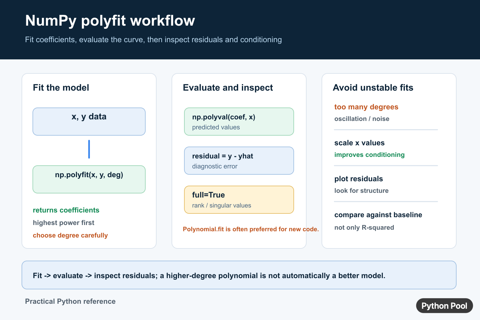
Call np.polyfit(x, y, degree) to obtain coefficients in descending power order. Use np.polyval(coefficients, x_values) to calculate predictions. Pass full=True when you need rank and singular-value diagnostics, and consider the newer Polynomial.fit() API for better numerical handling. The official NumPy polyfit reference documents the return values and warnings.
Fit a basic polynomial
The x and y arrays represent observed coordinates. The degree controls the model’s flexibility: degree one is a line, degree two is a quadratic, and higher degrees add more terms.
import numpy as np

x = np.array([0, 1, 2, 3])
y = np.array([1, 2, 5, 10])
coefficients = np.polyfit(x, y, deg=2)

print(coefficients)
The returned coefficients are ordered from the highest power to the constant term. For a quadratic, the result corresponds to a*x**2 + b*x + c. Keep this ordering in mind when passing coefficients to another function or displaying the fitted equation.
Evaluate the fitted curve
polyfit() does not return predicted y values. Use polyval() to evaluate the coefficient vector at the original x values or at a dense grid for plotting.
import numpy as np

x = np.array([0, 1, 2, 3])
y = np.array([1, 2, 5, 10])
coefficients = np.polyfit(x, y, 2)
predicted = np.polyval(coefficients, x)

print(predicted)
Evaluate on the observed points to calculate residuals. Evaluate on a new range only when interpolation or extrapolation is meaningful for the problem.
Inspect residuals instead of only the curve
A fit can look plausible while leaving a pattern in its residuals. Calculate y - predicted, plot the residuals against x, and check whether the errors are centered, whether their spread changes, or whether a systematic shape remains. Residual structure is evidence that the chosen degree or model may be missing something.
residuals = y - predicted
print(residuals)
print(np.mean(residuals))
Do not interpret a small average residual as proof of a good fit. Positive and negative errors can cancel, so inspect their distribution and scale as well.
Use full=True for diagnostics
With full=True, NumPy returns the coefficients plus residuals, rank, singular values, and the cutoff used for the effective rank. These values help identify underdetermined or poorly conditioned fits.
coefficients, diagnostics, rank, singular_values, cutoff = np.polyfit(
    x,
    y,
    deg=2,
    full=True,
)
print(rank, singular_values)
Capture the complete return tuple intentionally. Code that assumes the ordinary coefficient-only return shape will break when full=True is introduced.
Handle RankWarning and unstable fits
High-degree polynomials or poorly scaled x values can make the underlying Vandermonde system ill-conditioned. The resulting coefficients may be extremely sensitive to small changes in the data. A warning should prompt a model review, not simply be hidden.
Center or scale x values when appropriate, reduce the degree, collect more informative data, or use a model with a more suitable basis. The Polynomial.fit() interface can make scaling and later evaluation clearer for new code.
Use weights and covariance deliberately
If observations have different uncertainty, the optional weights can express that difference. A weight is part of the statistical assumption, not a way to make an inconvenient point disappear. Document how the weights were produced and verify that the fitted curve still represents the measurement process.
The covariance option can provide coefficient uncertainty estimates, but its interpretation depends on the noise model and scaling assumptions. Treat it as a diagnostic output rather than an automatic confidence interval for every prediction.
Avoid unexamined extrapolation
Polynomial fits can behave reasonably inside the observed x range and diverge quickly outside it. Mark extrapolated regions in charts, test them against domain knowledge, and avoid presenting a visually smooth curve as evidence for values the data never covered.
Choose the degree from the problem
A larger degree can reduce training error while increasing variance and sensitivity to noise. Start with the lowest degree that represents the known relationship, compare the residuals with a simpler baseline, and validate on data that was not used to choose the coefficients. A fit is a model of an assumption, not a replacement for one.
When the x values cover a large numerical range, shift or scale them before fitting and translate the result back only at a clearly documented boundary. Poor scaling can make the coefficient vector look extreme even when the curve appears visually reasonable.
Use weights for measurement uncertainty
The w argument can give more influence to observations with lower uncertainty. The weights should reflect the statistical model, such as inverse standard deviation, rather than arbitrary importance. Compare a weighted and unweighted fit when the choice materially affects the conclusion.
weights = np.array([1.0, 1.0, 0.5, 0.5])
weighted = np.polyfit(x, y, deg=2, w=weights)
print(weighted)
Keep the source and meaning of weights with the fitted artifact. A coefficient vector without its degree, x scaling, weights, and data range is difficult to reproduce or audit.
Prefer a stable basis for new work
The older coefficient interface is convenient for quick calculations, while Polynomial.fit() provides a class-oriented workflow with domain and window handling. Use the API that makes evaluation, conversion, and scaling clearest for the project, and record that choice in the analysis.
For related NumPy workflows, see reshape arrays, create ranges, and measure spread.
Frequently Asked Questions
What does NumPy polyfit() return?
np.polyfit() returns polynomial coefficients ordered from the highest power to the constant term for the requested degree.
How do I evaluate coefficients from polyfit()
Pass the coefficients and x values to np.polyval(), or use a NumPy polynomial class when you need a clearer fitted-model object.
How can I inspect a polynomial fit?
Compare predictions with measured values, plot residuals, and request full diagnostics when rank or conditioning may be a concern.
Why can a high-degree polyfit be unstable?
High-degree models can oscillate and amplify numerical noise, especially when x values are poorly scaled or the model is extrapolated.
