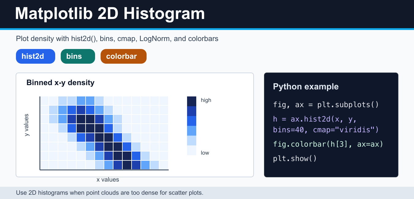
Matplotlib 2D Histogram: hist2d(), Bins, LogNorm, and Colorbars

Quick answer: A Matplotlib 2D histogram groups paired x and y observations into rectangular bins and displays the count in each bin as a colored grid. Choose bin edges and ranges deliberately, inspect the returned counts and edges, use LogNorm when counts are strongly skewed, and add a labeled colorbar before interpreting the picture.

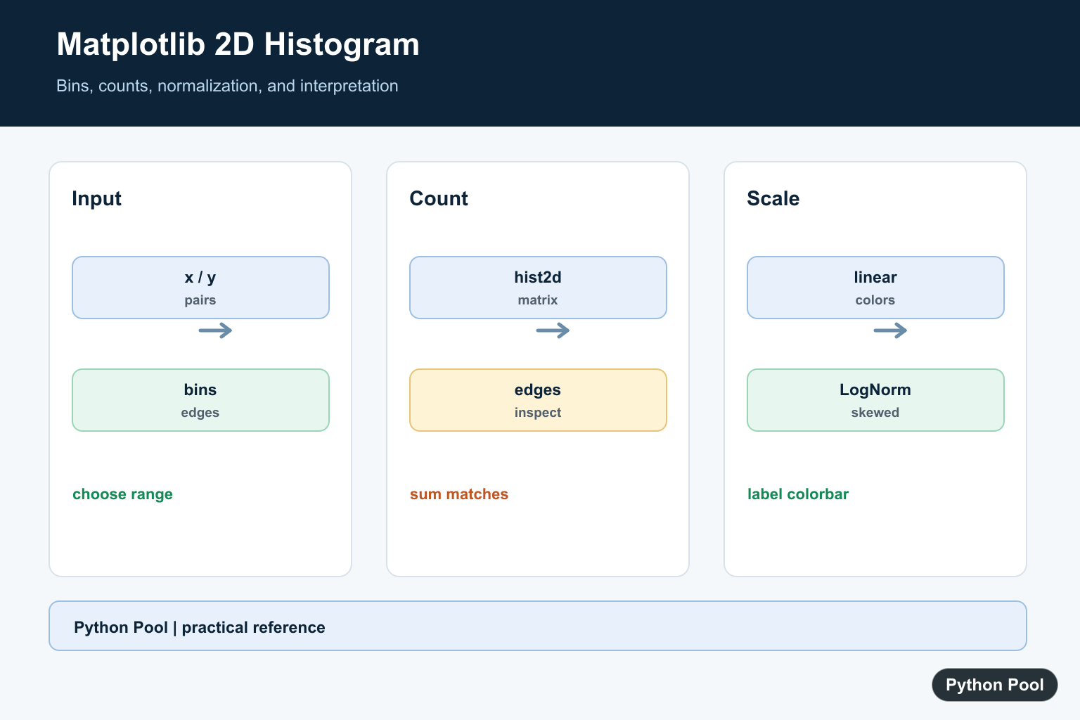
Python Pool infographic showing Matplotlib hist2d bins range LogNorm counts colorbar and dense point analysis — hist2d groups paired observations into rectangular bins; choose bin boundaries deliberately and use logarithmic normalization when counts are heavily skewed.

A Matplotlib 2D histogram counts how many points fall into each rectangular x-y bin. It is useful when a scatter plot has too many overlapping points and you want to see density instead of individual markers. In Matplotlib, the main helper is hist2d(), which returns the counts, x bin edges, y bin edges, and the image object used for the heatmap.

Use a 2D histogram for dense point clouds, paired measurements, simulation results, residual analysis, or any dataset where both x and y are numeric. If you only need a one-dimensional distribution, start with the PythonPool NumPy histogram guide.

Contents

Basic hist2d() example

The simplest example passes x values, y values, and a bin count. A colorbar is important because the color scale represents the number of points in each bin.

import numpy as np
import matplotlib.pyplot as plt

rng = np.random.default_rng(42)
x = rng.normal(size=5000)
y = 0.6 * x + rng.normal(scale=0.8, size=5000)

fig, ax = plt.subplots()
hist = ax.hist2d(x, y, bins=40, cmap="viridis")
fig.colorbar(hist[3], ax=ax, label="count")
ax.set_xlabel("x")
ax.set_ylabel("y")
ax.set_title("Matplotlib 2D histogram")
plt.show()

The returned tuple is commonly named hist or unpacked as counts, xedges, yedges, image. The image object is what you pass to fig.colorbar().

Control bins and range

The bins argument controls the resolution of the histogram. A small number of bins can hide structure; too many bins can make the plot noisy. You can pass one integer for both axes, a pair of integers, or explicit bin edges. Use range when you need a fixed visible area across multiple plots.

import numpy as np
import matplotlib.pyplot as plt

rng = np.random.default_rng(7)
x = rng.normal(loc=0, scale=1.2, size=8000)
y = rng.normal(loc=0, scale=0.7, size=8000)

fig, ax = plt.subplots()
hist = ax.hist2d(
    x,
    y,
    bins=(50, 30),
    range=[[-4, 4], [-3, 3]],
    cmap="magma",
)
fig.colorbar(hist[3], ax=ax, label="points per bin")
plt.show()

If the color scale is the main message, choose the colormap deliberately. The Matplotlib cmap guide explains built-in palettes, while the custom colormap guide covers building your own.

Python Pool infographic showing x and y samples, 2D bins, counts, edges, and a histogram grid — 2D bins: X and y samples, 2D bins, counts, edges, and a histogram grid.

Add LogNorm for skewed counts

Dense datasets often have a few bins with very high counts and many bins with low counts. A linear color scale can hide the low-density structure. Use matplotlib.colors.LogNorm when counts span a large range. Avoid it when zero-count bins are central to the story, because logarithmic normalization cannot display zero as a positive log value.

import numpy as np
import matplotlib.pyplot as plt
from matplotlib.colors import LogNorm

rng = np.random.default_rng(21)
x = rng.normal(size=20000)
y = x + rng.normal(scale=0.35, size=20000)

fig, ax = plt.subplots()
hist = ax.hist2d(x, y, bins=80, cmap="plasma", norm=LogNorm())
fig.colorbar(hist[3], ax=ax, label="log count")
plt.show()

Compute counts with NumPy histogram2d

Sometimes you need the counts before plotting. NumPy’s histogram2d() returns the count grid and bin edges without creating a figure. You can then plot the counts yourself or use them in another calculation.

import numpy as np

rng = np.random.default_rng(11)
x = rng.normal(size=1000)
y = rng.normal(size=1000)

counts, xedges, yedges = np.histogram2d(x, y, bins=20)
print(counts.shape)
print(xedges[:3])
print(yedges[:3])

For summary statistics around the same data, the PythonPool NumPy standard deviation guide can help with spread and variability.

Python Pool infographic mapping paired data through Matplotlib hist2d, counts, image, and axes — Plot hist2d: Paired data through Matplotlib hist2d, counts, image, and axes.

hist2d() vs hexbin()

hist2d() uses rectangular bins. hexbin() uses hexagonal bins. Rectangular bins are easier to align with grid-like data and fixed x-y ranges. Hexagonal bins often look smoother for natural point clouds because each bin has more even neighbor relationships. Try both when the visual conclusion depends on bin shape.

import numpy as np
import matplotlib.pyplot as plt

rng = np.random.default_rng(99)
x = rng.normal(size=6000)
y = 0.4 * x + rng.normal(size=6000)

fig, ax = plt.subplots()
plot = ax.hexbin(x, y, gridsize=45, cmap="viridis")
fig.colorbar(plot, ax=ax, label="count")
plt.show()

Common 2D histogram mistakes

Too few bins: the plot becomes blocky and hides detail.
Too many bins: random noise can look like structure.
No colorbar: readers cannot interpret the count scale.
Bad colormap choice: some palettes exaggerate small differences or hide extremes.
Different ranges across plots: comparisons become misleading if each chart auto-scales differently.

Use clear labels and a readable colorbar title. The Matplotlib colorbar guide covers tick labels and placement. When exporting final charts, use the Matplotlib savefig guide to avoid clipped labels.

How to choose bins for a 2D histogram

Bin choice changes the story a 2D histogram tells. Start with a moderate value such as bins=40 or bins=50, then test a smaller and larger value. If the same dense regions appear across several settings, the pattern is more likely to be meaningful. If the pattern disappears when the bin count changes, the chart may be showing binning noise rather than a real relationship.

Use a fixed range when comparing multiple groups. Otherwise, each chart can auto-scale to a different area and make two distributions look more similar or more different than they really are. Also decide whether outliers should be visible in the range or summarized separately. Extreme outliers can force most of the useful data into a small part of the plot.

When presenting the result, describe what one bin means: a rectangle covering a range of x values and a range of y values. The color is the count inside that rectangle, not the value of a single point. This distinction matters when readers are used to scatter plots.

Python Pool infographic comparing linear counts, LogNorm, colorbar, sparse bins, and contrast — Color scale: Linear counts, LogNorm, colorbar, sparse bins, and contrast.

Official references

Choose Bins And Range Deliberately

The number of bins changes the question the plot appears to answer. A coarse grid shows broad concentration, while a fine grid reveals detail but can look noisy. An explicit range also makes comparisons between datasets more stable.

import numpy as np
import matplotlib.pyplot as plt

rng = np.random.default_rng(7)
x = rng.normal(size=2_000)
y = 0.7 * x + rng.normal(scale=0.6, size=2_000)

fig, ax = plt.subplots()
hist, x_edges, y_edges, image = ax.hist2d(
    x, y, bins=(40, 30), range=[[-3, 3], [-3, 3]], cmap="viridis"
)
fig.colorbar(image, ax=ax, label="observations per bin")

Inspect The Returned Arrays

hist2d returns the count matrix, x edges, y edges, and the image object. Checking their shapes is useful when the plotted result will feed a later calculation or when a surprising picture may be caused by input clipping.

hist, x_edges, y_edges, image = ax.hist2d(x, y, bins=20)
print(hist.shape)
print(len(x_edges) - 1, len(y_edges) - 1)
print(hist.sum(), len(x))

Python Pool infographic testing empty data, ranges, bin edges, NaN values, and labels — Plot checks: Empty data, ranges, bin edges, NaN values, and labels.

Use LogNorm For Skewed Counts

A linear color scale can make low-count bins disappear when a few bins dominate. LogNorm changes the color mapping, not the underlying counts, so label the colorbar and remember that equal-looking color steps represent multiplicative changes.

from matplotlib.colors import LogNorm

fig, ax = plt.subplots()
hist, x_edges, y_edges, image = ax.hist2d(
    x, y, bins=40, norm=LogNorm(), cmap="magma"
)
fig.colorbar(image, ax=ax, label="count, logarithmic colors")

Compare hist2d And hexbin

hist2d uses rectangular bins and is a good fit when x and y intervals have direct meaning. hexbin uses hexagonal cells and can reduce directional artifacts in dense scatter data. Choose one, then keep its scale and limits consistent across comparisons.

fig, axes = plt.subplots(1, 2, figsize=(10, 4), constrained_layout=True)
axes[0].hist2d(x, y, bins=30, cmap="viridis")
axes[0].set_title("rectangular bins")
axes[1].hexbin(x, y, gridsize=30, mincnt=1, cmap="viridis")
axes[1].set_title("hexagonal bins")

Matplotlib documents Axes.hist2d(), including its returned arrays, bins, range, and normalization arguments. The hexbin() API explains the alternative cell geometry, while Figure.colorbar() connects the image to a readable scale. Related references include NumPy histograms and normal samples.

For related density and binning choices, compare NumPy histograms, colorbars, and normal samples before interpreting a 2D count grid.

Frequently Asked Questions

What is a Matplotlib 2D histogram?

It counts paired x-y observations inside rectangular bins and displays the counts as a colored density grid.

How do I choose bins for hist2d()?

Use domain knowledge, sample size, and the visual question to choose a bin count or explicit edges; compare the result at multiple resolutions when unsure.