Matplotlib contourf(): Levels, Colormaps, Colorbars, and Grids

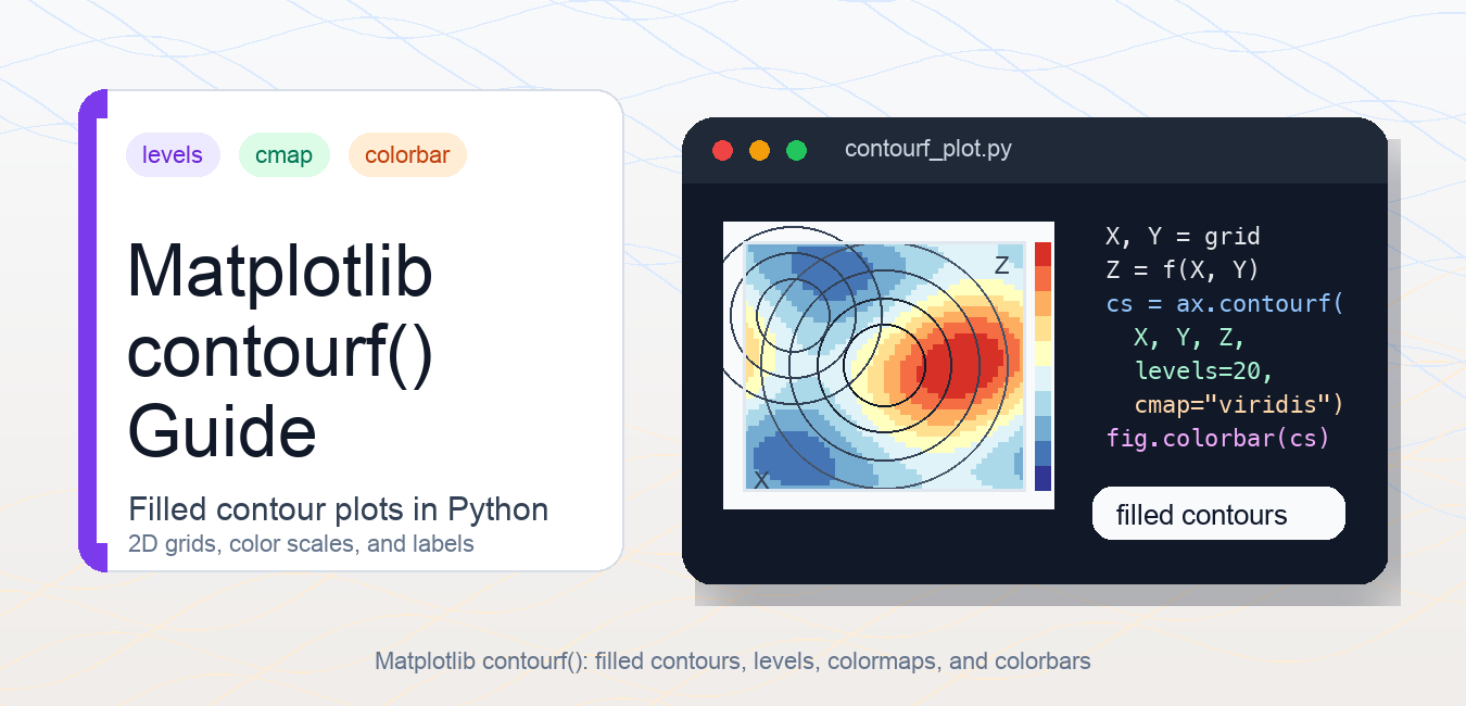
Quick answer: Matplotlib contourf() fills the regions between contour levels for a 2D value field. Give it compatible X, Y, and Z data, choose levels deliberately when comparisons matter, store the returned QuadContourSet, and connect that object to a labeled colorbar so the colors have an unambiguous meaning.

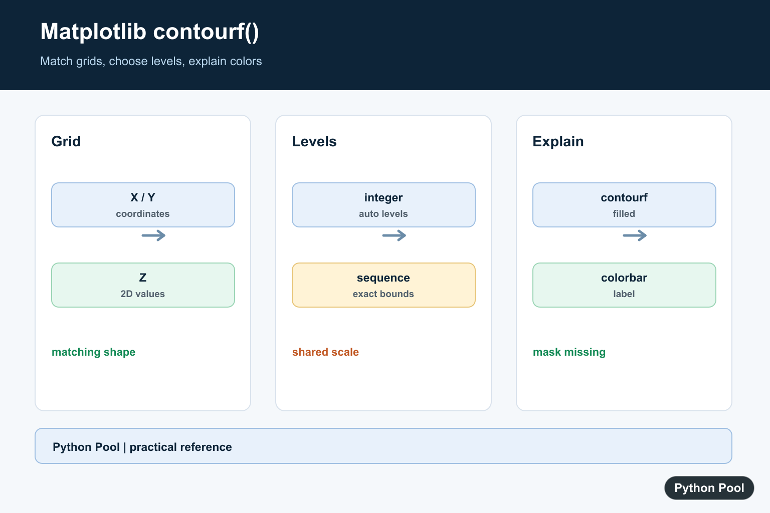
Matplotlib contourf() draws filled contour plots from a 2D grid of values. It is useful when you want to show how a value changes across two input variables, such as height over a map, loss over a parameter grid, or intensity over coordinates. Unlike contour(), which draws only contour lines, contourf() fills the areas between levels with color.

The usual workflow is simple: build X and Y coordinate arrays, compute a matching Z array, pass them to ax.contourf(), and add a colorbar so readers can interpret the colors.

Basic contourf example

Most examples start with NumPy arrays. np.meshgrid() turns one-dimensional x and y coordinates into two-dimensional coordinate grids. The Z array must match the shape of those grids.

import numpy as np
import matplotlib.pyplot as plt

x = np.linspace(-3, 3, 100)
y = np.linspace(-3, 3, 100)
X, Y = np.meshgrid(x, y)
Z = np.sin(X) * np.cos(Y)

fig, ax = plt.subplots()
filled = ax.contourf(X, Y, Z, levels=20, cmap="viridis")
fig.colorbar(filled, ax=ax, label="Z value")

ax.set_title("Filled contour plot")
ax.set_xlabel("X")
ax.set_ylabel("Y")
plt.show()

The levels argument controls how many contour bands appear. A larger value creates a smoother-looking plot; a smaller value makes the level boundaries easier to read. The cmap argument controls the color palette. For more on colormap choices, see the PythonPool guide to Matplotlib cmap.

Set explicit levels and colorbar range

When comparing several figures, avoid automatic levels because each plot may use a different scale. Instead, pass explicit levels. This makes the colors comparable across plots.

levels = np.linspace(-1, 1, 21)

fig, ax = plt.subplots()
filled = ax.contourf(
    X,
    Y,
    Z,
    levels=levels,
    cmap="RdBu_r",
    extend="both",
)
fig.colorbar(filled, ax=ax, label="Value")
plt.show()

The extend="both" option shows that values outside the first and last levels exist. That is helpful when you intentionally cap the range. If the colorbar itself is the part you need to customize, read Matplotlib colorbar examples.

Add contour lines on top of filled contours

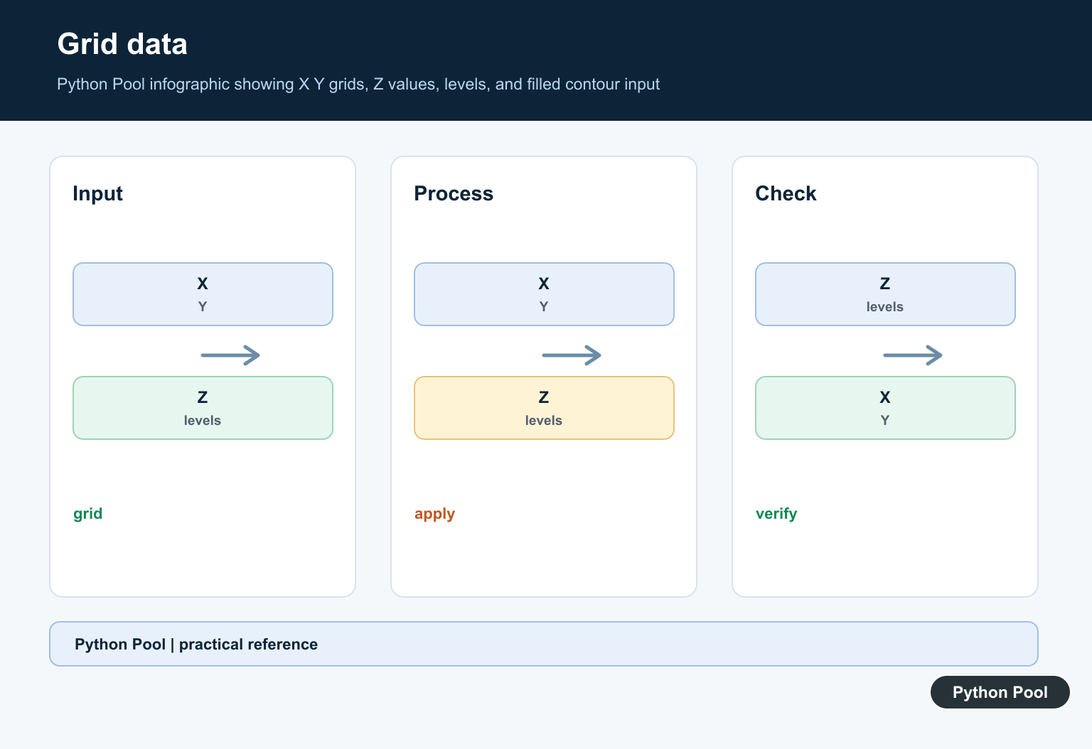
A filled contour plot can be beautiful but hard to read precisely. Add contour() on top when you want visible boundaries or labels. The two functions can use the same X, Y, Z, and levels.

fig, ax = plt.subplots()
filled = ax.contourf(X, Y, Z, levels=12, cmap="plasma")
lines = ax.contour(X, Y, Z, levels=12, colors="black", linewidths=0.6)
ax.clabel(lines, inline=True, fontsize=8)
fig.colorbar(filled, ax=ax)
plt.show()

Use this style for reports where the actual level boundaries matter. If your plot is based on rectangular cells instead of smooth contour interpolation, Matplotlib pcolormesh may be a better fit.

Use contourf with subplots

Filled contour plots often appear in side-by-side comparisons. Keep the color scale consistent by reusing the same levels across every subplot.

fig, axes = plt.subplots(1, 2, figsize=(8, 3), layout="constrained")
levels = np.linspace(-1, 1, 21)

for ax, scale in zip(axes, [1.0, 0.5]):
    filled = ax.contourf(X, Y, scale * Z, levels=levels, cmap="viridis")
    ax.set_title(f"scale={scale}")

fig.colorbar(filled, ax=axes, label="Value")
plt.show()

The shared colorbar helps readers compare the two panels. If labels or colorbars overlap, the refreshed guide to Matplotlib subplot spacing explains how to fix the layout.

3D filled contour projection

Matplotlib can also draw filled contours on a 3D axis. This is not the same as a full 3D surface; it is a filled contour projection placed on a plane. Use it when you want a contour map inside a 3D scene.

fig = plt.figure()
ax = fig.add_subplot(projection="3d")

ax.contourf(X, Y, Z, zdir="z", offset=-1.2, levels=20, cmap="viridis")
ax.plot_surface(X, Y, Z, cmap="viridis", alpha=0.55)

ax.set_zlim(-1.2, 1.2)
plt.show()

For vector-field plots that show direction rather than filled value regions, compare this with Matplotlib quiver. For styling and stacking multiple artists, Matplotlib zorder is also useful.

contourf() vs contour()

Use contourf() when the filled regions are the main message. Use contour() when the level lines themselves are the main message. In many scientific plots, the best result combines both: contourf() for color and contour() for readable boundaries or labels.

Common contourf mistakes

The most common mistake is passing arrays with incompatible shapes. If X and Y are two-dimensional, Z must have the same shape. If X and Y are one-dimensional, their lengths must match the columns and rows of Z. Another common issue is choosing too many levels, which can make the plot look smooth but hide meaningful boundaries. Start with 10 to 20 levels and increase only when the data supports it.

Also be careful with color maps. Sequential colormaps work well for values that move from low to high. Diverging colormaps work better when zero or a central baseline matters. Finally, always add a colorbar or the colors become hard to interpret. If you need to style the background around the axes, see Matplotlib background color.

Keep the plot readable by choosing meaningful levels, adding a colorbar, and labeling axes. If your figure uses grid lines, the Matplotlib grid guide covers axis grid styling separately from contour levels.

Official references

• Matplotlib pyplot.contourf documentation
• Matplotlib contour API
• Matplotlib pyplot.contour documentation
• Matplotlib pyplot.colorbar documentation
• Matplotlib colormap guide
• Matplotlib clabel documentation
• Matplotlib 3D contour example
• NumPy meshgrid documentation

Build A Matching X Y Z Grid

Z contains the values to fill. X and Y can be one-dimensional coordinate arrays or matching two-dimensional grids. The coordinate shape must describe the columns and rows of Z; a mismatch is a data-layout error, not a colormap problem.

import numpy as np
import matplotlib.pyplot as plt

x = np.linspace(-2, 2, 80)
y = np.linspace(-2, 2, 60)
X, Y = np.meshgrid(x, y)
Z = np.sin(X) * np.cos(Y)

fig, ax = plt.subplots()
filled = ax.contourf(X, Y, Z, levels=12, cmap="viridis")
fig.colorbar(filled, ax=ax, label="value")

Pass Explicit Levels For Comparisons

An integer asks Matplotlib to choose a number of levels. A sorted sequence gives exact boundaries, which is safer when two plots must use the same bins or when a threshold has domain meaning.

levels = [-1.0, -0.5, 0.0, 0.5, 1.0]
fig, ax = plt.subplots()
filled = ax.contourf(X, Y, Z, levels=levels, cmap="coolwarm", extend="both")
ax.contour(X, Y, Z, levels=levels, colors="black", linewidths=0.5)
fig.colorbar(filled, ax=ax, label="shared scale")

Use A Colorbar And Norm Together

A colorbar explains the mapping from values to colors. For skewed or positive data, a normalization object can make low values visible, but its limits and tick labels should match the question being answered.

from matplotlib.colors import LogNorm

positive = np.exp(-(X**2 + Y**2)) * 100 + 0.1
fig, ax = plt.subplots()
filled = ax.contourf(X, Y, positive, levels=20, norm=LogNorm(), cmap="magma")
fig.colorbar(filled, ax=ax, label="log-scaled value")

Handle Missing And Out-Of-Range Data

Mask invalid cells before plotting rather than silently turning missing values into meaningful colors. extend controls how values outside the supplied levels are represented, while a masked array keeps gaps visible in the field.

values = np.ma.masked_where((X**2 + Y**2) < 0.25, Z)
fig, ax = plt.subplots()
filled = ax.contourf(X, Y, values, levels=levels, cmap="viridis", extend="both")
fig.colorbar(filled, ax=ax)
ax.set_aspect("equal")

Read the official Axes.contourf() API for level, coordinate, colormap, and normalization behavior, and the Figure.colorbar() API for attaching a color scale. Related references include Matplotlib colorbars and custom colormaps.

For related filled-field presentation, compare colorbars, custom colormaps, and Gridspec layout when making a contour plot readable and comparable.

Frequently Asked Questions

What does Matplotlib contourf() do?

contourf() draws filled contour regions from a 2D Z array and optional X and Y coordinates, using levels and a colormap to represent value ranges.

What shapes must X, Y, and Z have?

X and Y can be matching 2D grids or compatible 1D coordinate arrays, while Z is a matching M-by-N value grid.

How do I choose contour levels?

Pass an increasing sequence when exact boundaries matter, or an integer when Matplotlib should choose a reasonable number of levels.

How do I add a colorbar to contourf?

Store the returned contour set and pass it to fig.colorbar() or plt.colorbar(), then label the colorbar so the value scale is clear.