Spectrogram in Python: Visualize Frequency Over Time

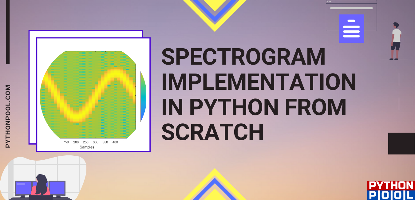
Quick answer: A spectrogram shows how signal energy changes across frequency and time. SciPy can compute it by applying a short-time Fourier transform to overlapping windows; the sampling rate, window length, overlap, and scale determine how the result should be interpreted.

A spectrogram shows how the frequency content of an audio signal changes over time. In Python, the most direct workflow is to load an audio file, compute a short-time Fourier transform, convert the magnitude to decibels, and display the result as an image. A spectrogram analyzes sound; on Windows, Python winsound Module Examples covers the standard-library playback side with aliases, WAV files, flags, and asynchronous calls.

This tutorial uses librosa, NumPy, and Matplotlib. The current librosa.stft() documentation describes STFT as a time-frequency representation computed over short overlapping windows. That is the core operation behind the spectrogram.

Install the Required Packages

Install the plotting and audio packages first:

python -m pip install librosa matplotlib numpy

Use a short .wav or .mp3 file while testing so the plot appears quickly.

Complete Spectrogram Code

Replace audio.wav with the path to your audio file:

import librosa
import librosa.display
import matplotlib.pyplot as plt
import numpy as np

AUDIO_FILE = "audio.wav"

y, sr = librosa.load(AUDIO_FILE, sr=None)

stft = librosa.stft(y)
spectrogram_db = librosa.amplitude_to_db(np.abs(stft), ref=np.max)

fig, ax = plt.subplots(figsize=(10, 4))
image = librosa.display.specshow(
    spectrogram_db,
    sr=sr,
    x_axis="time",
    y_axis="hz",
    ax=ax,
)

ax.set_title("Spectrogram")
fig.colorbar(image, ax=ax, format="%+2.0f dB")
plt.tight_layout()
plt.show()

How the Code Works

librosa.load() reads the audio file and returns two values: the audio samples and the sample rate. The official librosa.load() documentation notes that sr=None preserves the file’s native sampling rate instead of resampling to the default.

librosa.stft(y) converts the waveform into a complex-valued matrix. The magnitude of that matrix is calculated with np.abs(stft). If you want a broader refresher on magnitude calculations, see Python Pool’s guide to NumPy magnitude.

librosa.amplitude_to_db() converts the amplitude spectrogram into a decibel-scaled spectrogram. The official amplitude_to_db() reference describes it as a convenience function for converting amplitude values to dB. Using ref=np.max makes the loudest point 0 dB and shows quieter regions as negative values.

librosa.display.specshow() draws the matrix as an image with labeled axes. The specshow() documentation supports time labels on the x-axis and frequency labels such as hz or log on the y-axis.

Plot the Waveform First

A waveform plot is useful before creating the spectrogram because it shows silence, clipping, and rough duration. Current librosa display examples use librosa.display.waveshow() for this:

fig, ax = plt.subplots(figsize=(10, 3))
librosa.display.waveshow(y, sr=sr, ax=ax)
ax.set_title("Waveform")
plt.tight_layout()
plt.show()

For plot sizing and color controls, these Python Pool guides may help: Matplotlib figsize, Matplotlib colorbar, and Matplotlib tight_layout.

Choosing n_fft and hop_length

Two STFT parameters control how the spectrogram looks. n_fft sets the analysis window size, which affects frequency detail. hop_length sets how many samples separate adjacent frames, which affects time detail. A smaller hop length produces more time columns, while a larger FFT window can make frequency bands easier to separate.

stft = librosa.stft(y, n_fft=2048, hop_length=512)
spectrogram_db = librosa.amplitude_to_db(np.abs(stft), ref=np.max)

For speech, try a smaller n_fft such as 512 or 1024. For music, 2048 is a reasonable starting point. Keep the same sr and hop_length values when calling specshow() so the time axis is labeled correctly.

Use a Log Frequency Axis

For music and speech, a logarithmic frequency scale is often easier to read than a linear one. Change y_axis="hz" to y_axis="log":

image = librosa.display.specshow(
    spectrogram_db,
    sr=sr,
    x_axis="time",
    y_axis="log",
    ax=ax,
)

Common Spectrogram Mistakes

• Using outdated waveform-display code instead of waveshow().
• Forgetting np.abs() before converting STFT values to decibels.
• Mixing sample rates by loading one rate and plotting with another.
• Plotting a very long audio file without trimming it first.

Related reading: NumPy inverse FFT, NumPy sin, and Python data types.

Start With The Sampling Rate

The sampling frequency maps array samples to real time and limits the highest representable frequency to roughly half the sample rate. A wrong fs produces misleading time and frequency axes.

Choose Window Size

Short windows track rapid changes but provide less frequency resolution. Long windows resolve nearby frequencies better while blurring when those frequencies occurred. Choose nperseg for the question the plot must answer.

Use Overlap Intentionally

Overlapping windows make the time axis smoother and reduce gaps between estimates, at the cost of more computation. Keep the relationship between nperseg, noverlap, and the signal length explicit.

Read The Axes Correctly

The output contains frequencies, segment times, and spectral values. Confirm whether the signal is real, whether one-sided frequencies are returned, and whether the plotted amplitude represents power or magnitude.

Use Decibels Carefully

A log or decibel transform helps reveal weak components across a wide dynamic range. Add a small floor before taking a logarithm and label the colorbar so readers know what quantity is displayed.

Validate With Known Signals

Test a sine wave at a known frequency, a signal with two tones, a changing chirp, and silence. Check that peaks appear where expected before trusting a complex recording or production measurement.

Document Units And Preprocessing

Record whether the input was normalized, detrended, filtered, or converted to mono. Label seconds, hertz, and decibels on the final plot so a reader can reproduce the interpretation rather than guessing from colors.

The official SciPy spectrogram reference documents the parameters and outputs. Related Python Pool references include diagnostics and verification.

For related signal workflows, compare measurement diagnostics, known-signal tests, and array operations when interpreting a spectrogram.

Frequently Asked Questions

What is a spectrogram?

A spectrogram displays how signal energy is distributed across frequencies as the signal changes over time.

Which Python library creates a spectrogram?

SciPy’s signal tools provide a standard spectrogram function, while NumPy and Matplotlib support arrays and visualization.

What does nperseg change?

nperseg controls the window length and therefore the time-frequency tradeoff: longer windows improve frequency detail but reduce time detail.

Why use a logarithmic or decibel scale?

Audio and other signals can span a wide dynamic range, so a log scale often makes weaker frequency components visible alongside stronger ones.