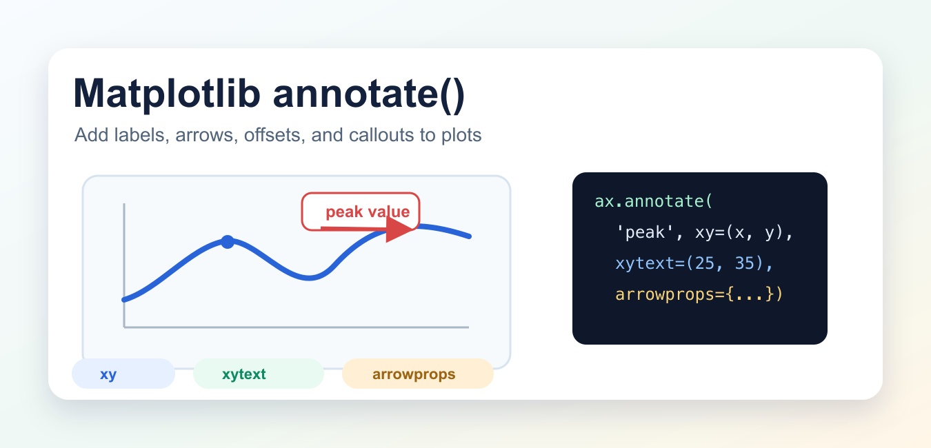
Matplotlib annotate(): Add Labels and Arrows to Plots

Quick answer: Matplotlib annotate() creates a callout attached to a coordinate. xy is the target point and xytext is the text position; arrowprops controls the connector. Keep coordinate systems, clipping, layout, and the final export size in mind so an annotation that looks correct interactively remains visible in a saved figure. A good annotation explains one decision or feature, not every point in a chart, so use labels selectively and keep the visual hierarchy readable.

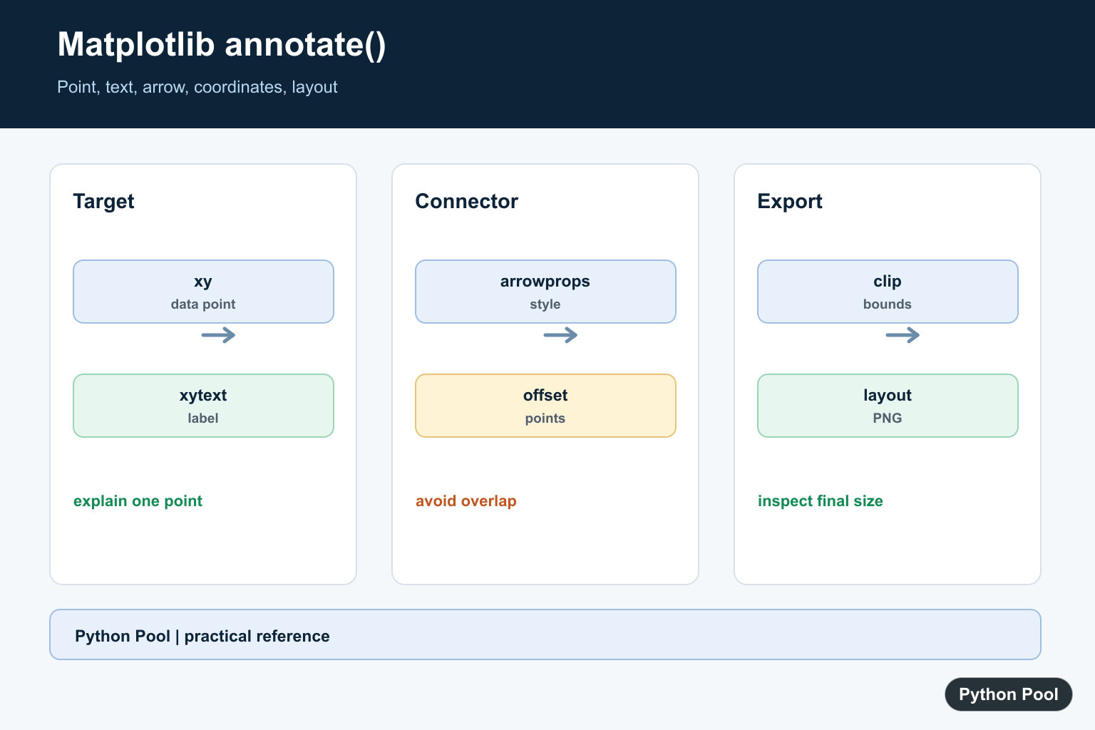
Python Pool infographic showing Matplotlib annotate text point xytext arrowprops coordinate systems and clipping — annotate() connects explanatory text to a data point; choose coordinates, offsets, arrows, and clipping so the callout remains readable.

matplotlib.annotate() adds explanatory text to a plot and can draw an arrow from that text to a specific data point. Use it when a chart needs a callout, peak label, threshold note, outlier explanation, or any label that should point to a plotted value. Annotations and legends label different chart elements; Fix No Handles With Labels Found in Legend fixes the case where legend() cannot find labeled artists.

In most object-oriented Matplotlib code, call ax.annotate(). The pyplot shortcut plt.annotate() works too, but using the Axes method is clearer when a figure has more than one subplot.

Contents

Basic Syntax

ax.annotate(
    text,
    xy,
    xytext=None,
    xycoords="data",
    textcoords=None,
    arrowprops=None,
    annotation_clip=None,
    **kwargs,
)

Argument	Purpose
`text`	The annotation label.
`xy`	The point being annotated. This is where the arrow points.
`xytext`	The text position. If omitted, the text is placed at `xy`.
`xycoords`	Coordinate system for `xy`. The default is `data`.
`textcoords`	Coordinate system for `xytext`.
`arrowprops`	Dictionary of arrow styling options. If omitted, no arrow is drawn.

Simple Annotation Example

This example labels the highest point of a sine curve. The annotation point uses data coordinates, while the text is offset from that point by 25 points horizontally and 35 points vertically.

import numpy as np
import matplotlib.pyplot as plt

x = np.linspace(0, 10, 100)
y = np.sin(x)
peak_index = np.argmax(y)

fig, ax = plt.subplots()
ax.plot(x, y)

ax.annotate(
    "peak",
    xy=(x[peak_index], y[peak_index]),
    xytext=(25, 35),
    textcoords="offset points",
    arrowprops={"arrowstyle": "->", "color": "crimson"},
)

plt.show()

The key detail is the difference between xy and xytext. xy identifies the data point. xytext controls where the label appears.

Python Pool infographic showing a Matplotlib point, annotation text, coordinates, and an arrow — Plot label: A Matplotlib point, annotation text, coordinates, and an arrow.

Add a Box Around the Label

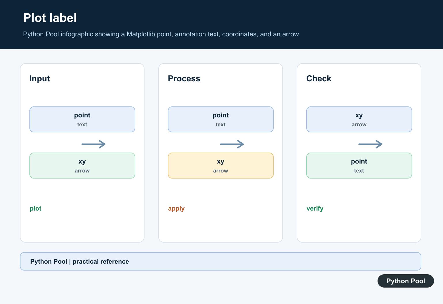
Because annotate() accepts text styling keyword arguments, you can add a background box with bbox and align the label with ha and va.

ax.annotate(
    "maximum value",
    xy=(x[peak_index], y[peak_index]),
    xytext=(30, 40),
    textcoords="offset points",
    ha="left",
    va="bottom",
    bbox={"boxstyle": "round,pad=0.3", "fc": "white", "ec": "crimson"},
    arrowprops={"arrowstyle": "->", "color": "crimson"},
)

This pattern is useful when the plotted line or background would make plain text hard to read.

Common Coordinate Systems

Matplotlib annotations are flexible because the arrow target and text can use different coordinate systems.

data: Uses the plotted data coordinates. This is the default for xy.
offset points: Places the text a fixed point offset from xy. This is common for labels that should follow a data point without covering it.
axes fraction: Uses the Axes box, where (0, 0) is bottom-left and (1, 1) is top-right.
figure fraction: Uses the full figure instead of a single Axes.

Annotation With Axes-Fraction Text

Sometimes the arrow should point to data, but the text should stay in a stable corner of the plot. Use xycoords="data" and textcoords="axes fraction".

ax.annotate(
    "important point",
    xy=(4, np.sin(4)),
    xycoords="data",
    xytext=(0.05, 0.95),
    textcoords="axes fraction",
    ha="left",
    va="top",
    arrowprops={"arrowstyle": "->", "connectionstyle": "arc3,rad=0.2"},
)

This keeps the label near the top-left of the Axes even if the data limits change.

Python Pool infographic mapping annotate arguments through arrow style, offset text, and target point — Arrow props: Annotate arguments through arrow style, offset text, and target point.

Styling Annotation Arrows

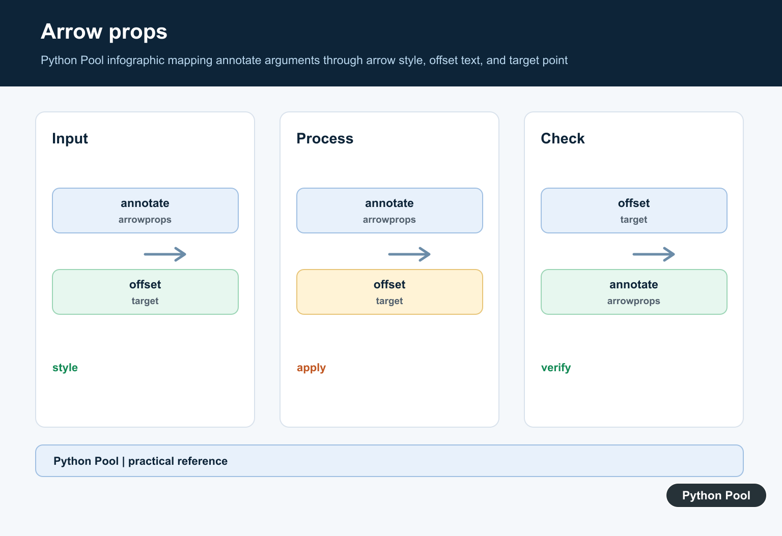
For modern Matplotlib code, prefer the fancy-arrow style by setting arrowstyle. You can also use connectionstyle for curved arrows.

arrowprops = {
    "arrowstyle": "->",
    "color": "black",
    "linewidth": 1.5,
    "connectionstyle": "arc3,rad=-0.2",
}

If you need standalone arrows rather than text annotations, see the related Matplotlib arrow guide.

Why Matplotlib annotate Is Not Showing

The point is outside the visible axis limits. Check ax.set_xlim() and ax.set_ylim(). The Matplotlib ylim guide covers y-axis limits in detail.
The text is clipped. Try moving xytext, using annotation_clip=False, or increasing the plot margins.
The arrow color blends into the chart. Set a visible color, linewidth, or bbox.
You annotated the wrong Axes. In multi-plot figures, call annotate() on the correct ax. The Matplotlib gca guide explains current Axes behavior.

Python Pool infographic comparing text offset, clipping, axes limits, overlapping labels, and layout — Keep readable: Text offset, clipping, axes limits, overlapping labels, and layout.

Related Matplotlib Guides

Annotations often pair well with shape and styling helpers. See how to draw circles in Matplotlib, how to change Matplotlib background color, and Matplotlib pcolormesh for more plotting examples.

Official References

Conclusion

Use ax.annotate() when a plot needs a clear callout. Set xy for the data point, xytext for the label position, textcoords for offsets, and arrowprops for arrows. These four options handle most annotation tasks cleanly.

Place Text At A Data Point

The simplest annotation uses data coordinates for both the target and text. This keeps the label tied to plotted values when the axes limits change. Use a short label and inspect crowded points before adding more callouts.

import matplotlib.pyplot as plt

fig, ax = plt.subplots()
x = [1, 2, 3, 4]
y = [2, 5, 3, 7]
ax.plot(x, y, marker="o")
ax.annotate("peak", xy=(4, 7))
fig.savefig("annotated.png", dpi=160)
plt.close(fig)

Separate xy And xytext

xy identifies what the annotation explains, while xytext identifies where the label sits. Moving text away from the point prevents overlap. arrowprops can add a visible connector and use an arrow style that survives the output size.

import matplotlib.pyplot as plt

fig, ax = plt.subplots()
ax.scatter([1, 2, 3], [2, 5, 3])
ax.annotate("highest value", xy=(2, 5), xytext=(2.4, 6), arrowprops={"arrowstyle": "->"})
fig.tight_layout()

Python Pool infographic testing transforms, multiple labels, savefig, resize, and rendered output — Annotation checks: Transforms, multiple labels, savefig, resize, and rendered output.

Choose Coordinate Systems

By default, xy and xytext use data coordinates. axes fraction, figure fraction, offset points, and other coordinate systems are useful when a label should stay near a corner or use a fixed visual offset. Set the coordinate systems explicitly when their meanings differ.

import matplotlib.pyplot as plt

fig, ax = plt.subplots()
ax.plot([0, 1], [0, 1])
ax.annotate("axes note", xy=(0.8, 0.8), xycoords="data", xytext=(0.05, 0.95), textcoords="axes fraction", arrowprops={"arrowstyle": "->"})

Prevent Clipping And Overlap

An annotation can be clipped by the axes, hidden behind another artist, or cut off by the saved bounding box. Use annotation_clip deliberately, reserve layout space, and render the final PNG or PDF at its actual dimensions. A label should explain data without covering the point or neighboring labels.

import matplotlib.pyplot as plt

fig, ax = plt.subplots(figsize=(6, 4), constrained_layout=True)
ax.plot([1, 2, 3], [1, 4, 2])
ax.annotate("callout", xy=(2, 4), xytext=(2.5, 4.5), annotation_clip=False)
fig.savefig("callout.png", dpi=160, bbox_inches="tight")
plt.close(fig)

Matplotlib’s official Axes.annotate() reference defines xy, xytext, coordinate systems, arrowprops, and clipping. Treat annotations as part of the figure layout, not as an afterthought added after export.

For related chart labeling and layout, compare legend handle fixes, current Axes inspection, and vertical plot markers when placing callouts that should remain readable.